

268
M. Méndez and T. M. Belloni
PDS. This is so because the amplitude of the variability of the pulsar signal is spread
over all time bins in the light curve, but the power is concentrated in a few frequency
bins (ideally one) in a PDS. The same applies to signals that are not strictly periodic;
the advantage in these cases is, again, that in the PDS one can isolate, and study
separately, the properties of different variability components that are present in the
light curve, but span only a limited range of frequencies, whereas this is impossible
using the light curve directly. Also because of this, one final advantage of using the
PDS is that, at each frequency, one can easily separate and subtract the part of the
variability in the light curve due to the Poisson nature of the signal. The power per
unit frequency of a constant, Poisson dominated, signal is also a constant that, when
the units of the PDS are chosen conveniently [90], is equal to 2. In the remainder of
this chapter we will use the PDS to characterise the variability components observed
in accreting X-ray sources.
Without entering into too much details, a PDS gives the power per unit frequency
of a signal as a function of frequency. The units of the power can be chosen
arbitrarily, but the important point we want to make here is that this power is per
unit frequency (therefore the word density in the name power density spectrum; as
is common in the literature, here we use loosely the word power to refer to power
density). The total power in a light curve over a certain range of time scales is
the integral of the PDS with respect to frequency over the corresponding range of
frequencies; this quantity is no longer a density (per unit frequency) and, because
of Parseval’s theorem, this integral is equal to the total variance in the light curve
in that particular frequency range. By choosing the appropriate PDS normalisation,
this quantity can represent the fractional root-mean square variability, also known as
fractional rms, in the light curve over a range of frequencies (see [161], for details).
After producing the PDS of a light curve, the power can be fitted as a function
of frequency with (a combination of) all kinds of mathematical functions, and use
the parameters of those functions to characterise the properties of the components
that those functions represent. Ideally those functions would have some underlying
theoretical meaning but, even if they do not, one can still deduce interesting
properties of the processes that produce that variability, and eventually about
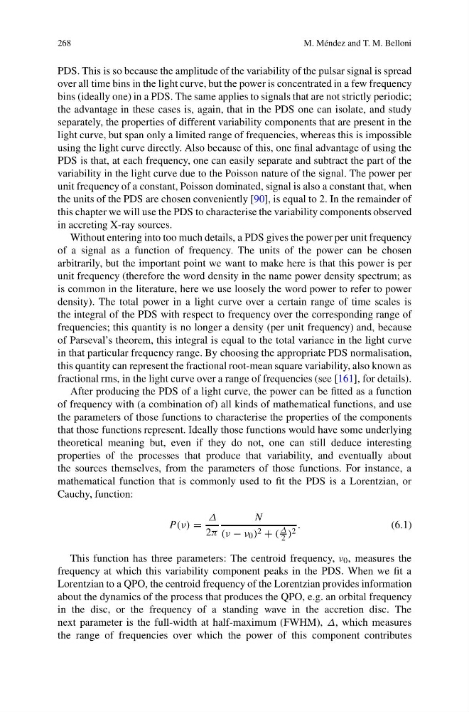
the sources themselves, from the parameters of those functions. For instance, a
mathematical function that is commonly used to fit the PDS is a Lorentzian, or
Cauchy, function:
P (ν) =
Δ
2π
N
(ν − ν 0 ) 2 + (
Δ
2 ) 2
.
(6.1)
This function has three parameters: The centroid frequency, ν 0 , measures the
frequency at which this variability component peaks in the PDS. When we fit a
Lorentzian to a QPO, the centroid frequency of the Lorentzian provides information
about the dynamics of the process that produces the QPO, e.g. an orbital frequency
in the disc, or the frequency of a standing wave in the accretion disc. The
next parameter is the full-width at half-maximum (FWHM), Δ, which measures
the range of frequencies over which the power of this component contributes
M. Méndez and T. M. Belloni
PDS. This is so because the amplitude of the variability of the pulsar signal is spread
over all time bins in the light curve, but the power is concentrated in a few frequency
bins (ideally one) in a PDS. The same applies to signals that are not strictly periodic;
the advantage in these cases is, again, that in the PDS one can isolate, and study
separately, the properties of different variability components that are present in the
light curve, but span only a limited range of frequencies, whereas this is impossible
using the light curve directly. Also because of this, one final advantage of using the
PDS is that, at each frequency, one can easily separate and subtract the part of the
variability in the light curve due to the Poisson nature of the signal. The power per
unit frequency of a constant, Poisson dominated, signal is also a constant that, when
the units of the PDS are chosen conveniently [90], is equal to 2. In the remainder of
this chapter we will use the PDS to characterise the variability components observed
in accreting X-ray sources.
Without entering into too much details, a PDS gives the power per unit frequency
of a signal as a function of frequency. The units of the power can be chosen
arbitrarily, but the important point we want to make here is that this power is per
unit frequency (therefore the word density in the name power density spectrum; as
is common in the literature, here we use loosely the word power to refer to power
density). The total power in a light curve over a certain range of time scales is
the integral of the PDS with respect to frequency over the corresponding range of
frequencies; this quantity is no longer a density (per unit frequency) and, because
of Parseval’s theorem, this integral is equal to the total variance in the light curve
in that particular frequency range. By choosing the appropriate PDS normalisation,
this quantity can represent the fractional root-mean square variability, also known as
fractional rms, in the light curve over a range of frequencies (see [161], for details).
After producing the PDS of a light curve, the power can be fitted as a function
of frequency with (a combination of) all kinds of mathematical functions, and use
the parameters of those functions to characterise the properties of the components
that those functions represent. Ideally those functions would have some underlying
theoretical meaning but, even if they do not, one can still deduce interesting
properties of the processes that produce that variability, and eventually about
the sources themselves, from the parameters of those functions. For instance, a
mathematical function that is commonly used to fit the PDS is a Lorentzian, or
Cauchy, function:
P (ν) =
Δ
2π
N
(ν − ν 0 ) 2 + (
Δ
2 ) 2
.
(6.1)
This function has three parameters: The centroid frequency, ν 0 , measures the
frequency at which this variability component peaks in the PDS. When we fit a
Lorentzian to a QPO, the centroid frequency of the Lorentzian provides information
about the dynamics of the process that produces the QPO, e.g. an orbital frequency
in the disc, or the frequency of a standing wave in the accretion disc. The
next parameter is the full-width at half-maximum (FWHM), Δ, which measures
the range of frequencies over which the power of this component contributes