

4 Accreting Millisecond X-ray Pulsars
175
even if they are true variations of the NS rotation. This should be expected if, for
example, the accretion torques exhibit stochastic variations.
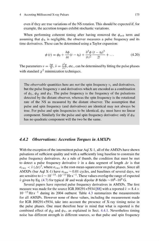
When performing coherent timing after having removed the φ orb term and
assuming that φ A is negligible, the observer measures a pulse frequency and its
time derivatives. These can be determined using a Taylor expansion:
φ (t) = φ 0 +
∂φ
∂t
(t − t 0 ) +
∂ 2 φ
∂ t 2
(t − t 0 ) 2
2!
+ . . .
(4.20)
The parameters ν =
∂φ
∂t , ˙
ν =
∂ 2 φ
∂ t 2 , etc., can be determined by fitting the pulse phases
with standard χ 2 minimization techniques.
The observable quantities here are not the spin frequency ν s and derivatives,
but the pulse frequency ν and derivatives which are encoded as a combination
of φ L , φ Q and φ N . The pulse frequency is the frequency of the pulsations
detected by the distant observer, whereas the spin frequency is the rotational
rate of the NS as measured by the distant observer. The assumption that
pulse and spin frequency (and derivatives) are identical may not always be
true. For pulse and spin frequencies to be identical, φ N must have no linear
component. Similarly for the pulse and spin frequency derivative: only if φ N
has no quadratic component will the two be the same.
4.4.2 Observations: Accretion Torques in AMXPs
With the exception of the intermittent pulsar Aql X-1, all of the AMXPs have shown
pulsations of sufficient quality and with a sufficiently long baseline to constrain the
pulse frequency derivatives. As a rule of thumb, the condition that must be met
to detect a pulse frequency derivative ˙
ν in a data segment of length Δt is that
σ rms < ˙
ν (Δt)
2 , where σ rms is the root-mean-square error on pulse phases. Since all
AMXPs (bar Aql X-1) have σ rms ∼ 0.01 cycles, and baselines of several days, we
are sensitive to ˙
ν ∼ 10 −15 –10 −13 Hz s −1 . These values overlap the range of expected
˙
ν given by Eq. (4.7) for typical ˙
M and weak dipolar B fields ∼10 8 –10 9 G.
Several papers have reported pulse frequency derivatives in AMXPs. The first
measure was made for the source IGR J00291+5934 [88] with a reported ˙
ν = 8.4 ×
10 −13 Hz s −1 during its 2004 outburst. Table 4.3 summarizes the measurements
for all AMXPs. However none of these values, including the measurement made
for IGR J00291+5934, take into account the presence of X-ray timing noise in
the pulse phases. One must therefore bear in mind that what is reported is the
combined effect of φ Q and φ N , as explained in Sect. 4.4.1. Nevertheless timing
noise has different strength in different sources, so that pulse and spin frequency
175
even if they are true variations of the NS rotation. This should be expected if, for
example, the accretion torques exhibit stochastic variations.
When performing coherent timing after having removed the φ orb term and
assuming that φ A is negligible, the observer measures a pulse frequency and its
time derivatives. These can be determined using a Taylor expansion:
φ (t) = φ 0 +
∂φ
∂t
(t − t 0 ) +
∂ 2 φ
∂ t 2
(t − t 0 ) 2
2!
+ . . .
(4.20)
The parameters ν =
∂φ
∂t , ˙
ν =
∂ 2 φ
∂ t 2 , etc., can be determined by fitting the pulse phases
with standard χ 2 minimization techniques.
The observable quantities here are not the spin frequency ν s and derivatives,
but the pulse frequency ν and derivatives which are encoded as a combination
of φ L , φ Q and φ N . The pulse frequency is the frequency of the pulsations
detected by the distant observer, whereas the spin frequency is the rotational
rate of the NS as measured by the distant observer. The assumption that
pulse and spin frequency (and derivatives) are identical may not always be
true. For pulse and spin frequencies to be identical, φ N must have no linear
component. Similarly for the pulse and spin frequency derivative: only if φ N
has no quadratic component will the two be the same.
4.4.2 Observations: Accretion Torques in AMXPs
With the exception of the intermittent pulsar Aql X-1, all of the AMXPs have shown
pulsations of sufficient quality and with a sufficiently long baseline to constrain the
pulse frequency derivatives. As a rule of thumb, the condition that must be met
to detect a pulse frequency derivative ˙
ν in a data segment of length Δt is that
σ rms < ˙
ν (Δt)
2 , where σ rms is the root-mean-square error on pulse phases. Since all
AMXPs (bar Aql X-1) have σ rms ∼ 0.01 cycles, and baselines of several days, we
are sensitive to ˙
ν ∼ 10 −15 –10 −13 Hz s −1 . These values overlap the range of expected
˙
ν given by Eq. (4.7) for typical ˙
M and weak dipolar B fields ∼10 8 –10 9 G.
Several papers have reported pulse frequency derivatives in AMXPs. The first
measure was made for the source IGR J00291+5934 [88] with a reported ˙
ν = 8.4 ×
10 −13 Hz s −1 during its 2004 outburst. Table 4.3 summarizes the measurements
for all AMXPs. However none of these values, including the measurement made
for IGR J00291+5934, take into account the presence of X-ray timing noise in
the pulse phases. One must therefore bear in mind that what is reported is the
combined effect of φ Q and φ N , as explained in Sect. 4.4.1. Nevertheless timing
noise has different strength in different sources, so that pulse and spin frequency