

972
Appendix: All Solutions to the Problems
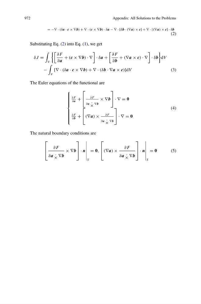
= −∇ · (δa · c × ∇b) + ∇ · (c × ∇b) · δa − ∇ · [δb · (∇ a) × c] + ∇ · [(∇ a) × c] · δb
(2)
Substituting Eq. (2) into Eq. (1), we get
δ J =
V
∂ F
∂ a
+ (c × ∇b) · ∇
· δa +
∂ F
∂ b
+ (∇ a × c) · ∇
· δb
dV
−
V
[∇ · (δa · c × ∇b) + ∇ · (δb · ∇a × c)]dV
(3)
The Euler equations of the functional are
⎧
⎪ ⎪ ⎪ ⎪ ⎪ ⎪ ⎨
⎪ ⎪ ⎪ ⎪ ⎪ ⎪ ⎩
∂ F
∂ a
+
⎡
⎣ ∂ F
∂ a ·
×
∇ b
× ∇b
⎤
⎦ · ∇ = 0
∂ F
∂ b
+
⎡
⎣ (∇ a) ×
∂ F
∂ a ·
×
∇ b
⎤
⎦ · ∇ = 0
(4)
The natural boundary conditions are
⎡
⎢
⎣
∂ F
∂ a ·
× ∇ b
× ∇b
⎤
⎥
⎦ · n
S
= 0,
⎡
⎢
⎣(∇ a) ×
∂ F
∂ a ·
× ∇ b
⎤
⎥
⎦ · n
S
= 0
(5)
Appendix: All Solutions to the Problems
= −∇ · (δa · c × ∇b) + ∇ · (c × ∇b) · δa − ∇ · [δb · (∇ a) × c] + ∇ · [(∇ a) × c] · δb
(2)
Substituting Eq. (2) into Eq. (1), we get
δ J =
V
∂ F
∂ a
+ (c × ∇b) · ∇
· δa +
∂ F
∂ b
+ (∇ a × c) · ∇
· δb
dV
−
V
[∇ · (δa · c × ∇b) + ∇ · (δb · ∇a × c)]dV
(3)
The Euler equations of the functional are
⎧
⎪ ⎪ ⎪ ⎪ ⎪ ⎪ ⎨
⎪ ⎪ ⎪ ⎪ ⎪ ⎪ ⎩
∂ F
∂ a
+
⎡
⎣ ∂ F
∂ a ·
×
∇ b
× ∇b
⎤
⎦ · ∇ = 0
∂ F
∂ b
+
⎡
⎣ (∇ a) ×
∂ F
∂ a ·
×
∇ b
⎤
⎦ · ∇ = 0
(4)
The natural boundary conditions are
⎡
⎢
⎣
∂ F
∂ a ·
× ∇ b
× ∇b
⎤
⎥
⎦ · n
S
= 0,
⎡
⎢
⎣(∇ a) ×
∂ F
∂ a ·
× ∇ b
⎤
⎥
⎦ · n
S
= 0
(5)