

894
Appendix: All Solutions to the Problems
1
0
(2 − 2x + x
2
)a 1 +
2 + 4x − x
2
+
2
3
x
3
a 2 − x + x
2
(2x − x
2
)dx = 0
1
0
(2 − 2x + x
2
)a 1 +
2 + 4x − x
2
+
2
3
x
3
a 2 − x + x
2
x
2
−
2
3
x
3
dx = 0
Integrating, we get
4
5
a 1 +
17
90
a 2 −
7
60
= 0
17
90
a 1 +
29
315
a 2 −
1
36
= 0
Solve a 1 and a 2
a 1 =
623
4306
= 0.1446818, a 2 =
21
4306
= 0.0048769
Therefore, the second approximate solution is
y 2 = x +
623
4306
x(2 − x) +
21
4306
x
2
1 −
2
3
x
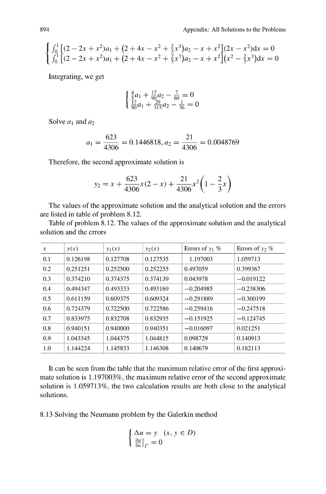
The values of the approximate solution and the analytical solution and the errors
are listed in table of problem 8.12.
Table of problem 8.12. The values of the approximate solution and the analytical
solution and the errors
x
y(x)
y 1 (x)
y 2 (x)
Errors of y 1 %
Errors of y 2 %
0.1
0.126198
0.127708
0.127535
1.197003
1.059713
0.2
0.251251
0.252500
0.252255
0.497059
0.399367
0.3
0.374210
0.374375
0.374139
0.043978
−0.019122
0.4
0.494347
0.493333
0.493169
−0.204985
−0.238306
0.5
0.611159
0.609375
0.609324
−0.291889
−0.300199
0.6
0.724379
0.722500
0.722586
−0.259416
−0.247518
0.7
0.833975
0.832708
0.832935
−0.151925
−0.124745
0.8
0.940151
0.940000
0.940351
−0.016097
0.021251
0.9
1.043345
1.044375
1.044815
0.098729
0.140913
1.0
1.144224
1.145833
1.146308
0.140679
0.182113
It can be seen from the table that the maximum relative error of the first approximate solution is 1.197003%, the maximum relative error of the second approximate
solution is 1.059713%, the two calculation results are both close to the analytical
solutions.
8.13 Solving the Neumann problem by the Galerkin method
u = y (x, y ∈ D)
∂u
∂n
Γ
= 0
Appendix: All Solutions to the Problems
1
0
(2 − 2x + x
2
)a 1 +
2 + 4x − x
2
+
2
3
x
3
a 2 − x + x
2
(2x − x
2
)dx = 0
1
0
(2 − 2x + x
2
)a 1 +
2 + 4x − x
2
+
2
3
x
3
a 2 − x + x
2
x
2
−
2
3
x
3
dx = 0
Integrating, we get
4
5
a 1 +
17
90
a 2 −
7
60
= 0
17
90
a 1 +
29
315
a 2 −
1
36
= 0
Solve a 1 and a 2
a 1 =
623
4306
= 0.1446818, a 2 =
21
4306
= 0.0048769
Therefore, the second approximate solution is
y 2 = x +
623
4306
x(2 − x) +
21
4306
x
2
1 −
2
3
x
The values of the approximate solution and the analytical solution and the errors
are listed in table of problem 8.12.
Table of problem 8.12. The values of the approximate solution and the analytical
solution and the errors
x
y(x)
y 1 (x)
y 2 (x)
Errors of y 1 %
Errors of y 2 %
0.1
0.126198
0.127708
0.127535
1.197003
1.059713
0.2
0.251251
0.252500
0.252255
0.497059
0.399367
0.3
0.374210
0.374375
0.374139
0.043978
−0.019122
0.4
0.494347
0.493333
0.493169
−0.204985
−0.238306
0.5
0.611159
0.609375
0.609324
−0.291889
−0.300199
0.6
0.724379
0.722500
0.722586
−0.259416
−0.247518
0.7
0.833975
0.832708
0.832935
−0.151925
−0.124745
0.8
0.940151
0.940000
0.940351
−0.016097
0.021251
0.9
1.043345
1.044375
1.044815
0.098729
0.140913
1.0
1.144224
1.145833
1.146308
0.140679
0.182113
It can be seen from the table that the maximum relative error of the first approximate solution is 1.197003%, the maximum relative error of the second approximate
solution is 1.059713%, the two calculation results are both close to the analytical
solutions.
8.13 Solving the Neumann problem by the Galerkin method
u = y (x, y ∈ D)
∂u
∂n
Γ
= 0