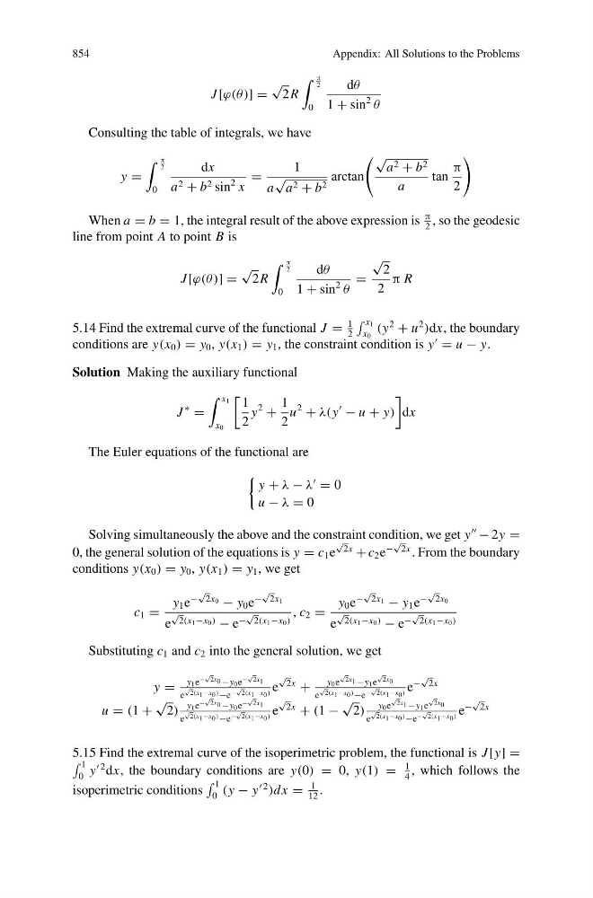
854
Appendix: All Solutions to the Problems
J [ϕ(θ)] =
√
2R
π
2
0
dθ
1 + sin
2
θ
Consulting the table of integrals, we have
y =
π
2
0
dx
a 2 + b 2 sin
2 x
=
1
a
√
a 2 + b 2
arctan
√
a 2 + b 2
a
tan
π
2
When a = b = 1, the integral result of the above expression is
π
2
, so the geodesic
line from point A to point B is
J [ϕ(θ)] =
√
2R
π
2
0
dθ
1 + sin
2
θ
=
√
2
2
π R
5.14 Find the extremal curve of the functional J =
1
2
x 1
x 0
(y
2
+ u
2
)dx, the boundary
conditions are y(x 0 ) = y 0 , y(x 1 ) = y 1 , the constraint condition is y
= u − y.
Solution Making the auxiliary functional
J
∗
=
x 1
x 0
1
2
y
2
+
1
2
u
2
+ λ(y
− u + y)
dx
The Euler equations of the functional are
y + λ − λ
= 0
u − λ = 0
Solving simultaneously the above and the constraint condition, we get y
− 2y =
0, the general solution of the equations is y = c 1 e
√
2x
+ c 2 e
−
√
2x . From the boundary
conditions y(x 0 ) = y 0 , y(x 1 ) = y 1 , we get
c 1 =
y 1 e
−
√
2x 0 − y 0 e
−
√
2x 1
e
√
2(x 1 −x 0 ) − e −
√
2(x 1 −x 0 )
, c 2 =
y 0 e
−
√
2x 1 − y 1 e
−
√
2x 0
e
√
2(x 1 −x 0 ) − e −
√
2(x 1 −x 0 )
Substituting c 1 and c 2 into the general solution, we get
y =
y 1 e
−
√
2x 0 −y 0 e
−
√
2x 1
e
√
2(x 1 −x 0 ) −e −
√
2(x 1 −x 0 )
e
√
2x
+
y 0 e
√
2x 1 −y 1 e
√
2x 0
e
√
2(x 1 −x 0 ) −e −
√
2(x 1 −x 0 )
e
−
√
2x
u = (1 +
√
2)
y 1 e
−
√
2x 0 −y 0 e
−
√
2x 1
e
√
2(x 1 −x 0 ) −e −
√
2(x 1 −x 0 )
e
√
2x
+ (1 −
√
2)
y 0 e
√
2x 1 −y 1 e
√
2x 0
e
√
2(x 1 −x 0 ) −e −
√
2(x 1 −x 0 )
e
−
√
2x
5.15 Find the extremal curve of the isoperimetric problem, the functional is J [y] =
1
0 y
2 dx, the boundary conditions are y(0) = 0, y(1) =
1
4
, which follows the
isoperimetric conditions
1
0 (y − y
2
)dx =
1
12
.