

Appendix: All Solutions to the Problems
851
c 1 and c 2 can be determined by the endpoint conditions, there c 2 = 0.
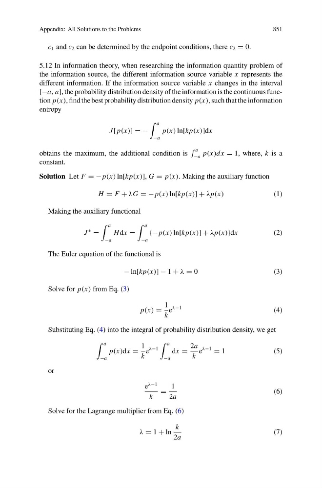
5.12 In information theory, when researching the information quantity problem of
the information source, the different information source variable x represents the
different information. If the information source variable x changes in the interval
[−a, a], the probability distribution density of the information is the continuous function p(x), find the best probability distribution density p(x), such that the information
entropy
J [ p(x)] = −
a
−a
p(x) ln[kp(x)]dx
obtains the maximum, the additional condition is
a
−a p(x)dx = 1, where, k is a
constant.
Solution Let F = −p(x) ln[kp(x)], G = p(x). Making the auxiliary function
H = F + λG = −p(x) ln[kp(x)] + λp(x)
(1)
Making the auxiliary functional
J
∗
=
a
−a
H dx =
a
−a
{− p(x) ln[kp(x)] + λp(x)}dx
(2)
The Euler equation of the functional is
− ln[kp(x)] − 1 + λ = 0
( 3 )
Solve for p(x) from Eq. (3)
p(x) =
1
k
e
λ−1
(4)
Substituting Eq. (4) into the integral of probability distribution density, we get
a
−a
p(x)dx =
1
k
e
λ−1
a
−a
dx =
2a
k
e
λ−1
= 1
( 5 )
or
e
λ−1
k
=
1
2a
(6)
Solve for the Lagrange multiplier from Eq. (6)
λ = 1 + ln
k
2a
(7)
851
c 1 and c 2 can be determined by the endpoint conditions, there c 2 = 0.
5.12 In information theory, when researching the information quantity problem of
the information source, the different information source variable x represents the
different information. If the information source variable x changes in the interval
[−a, a], the probability distribution density of the information is the continuous function p(x), find the best probability distribution density p(x), such that the information
entropy
J [ p(x)] = −
a
−a
p(x) ln[kp(x)]dx
obtains the maximum, the additional condition is
a
−a p(x)dx = 1, where, k is a
constant.
Solution Let F = −p(x) ln[kp(x)], G = p(x). Making the auxiliary function
H = F + λG = −p(x) ln[kp(x)] + λp(x)
(1)
Making the auxiliary functional
J
∗
=
a
−a
H dx =
a
−a
{− p(x) ln[kp(x)] + λp(x)}dx
(2)
The Euler equation of the functional is
− ln[kp(x)] − 1 + λ = 0
( 3 )
Solve for p(x) from Eq. (3)
p(x) =
1
k
e
λ−1
(4)
Substituting Eq. (4) into the integral of probability distribution density, we get
a
−a
p(x)dx =
1
k
e
λ−1
a
−a
dx =
2a
k
e
λ−1
= 1
( 5 )
or
e
λ−1
k
=
1
2a
(6)
Solve for the Lagrange multiplier from Eq. (6)
λ = 1 + ln
k
2a
(7)