

802
Appendix: All Solutions to the Problems
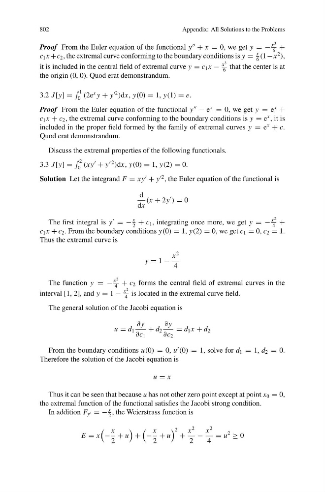
Proof From the Euler equation of the functional y
+ x = 0, we get y = −
x
3
6
+
c 1 x +c 2 , the extremal curve conforming to the boundary conditions is y =
x
6
(1−x
2
),
it is included in the central field of extremal curve y = c 1 x −
x
3
6
that the center is at
the origin (0, 0). Quod erat demonstrandum.
3.2 J [y] =
1
0 (2e
x y + y
2
)dx, y(0) = 1, y(1) = e.
Proof From the Euler equation of the functional y
− e
x
= 0, we get y = e
x
+
c 1 x + c 2 , the extremal curve conforming to the boundary conditions is y = e
x , it is
included in the proper field formed by the family of extremal curves y = e
x
+ c.
Quod erat demonstrandum.
Discuss the extremal properties of the following functionals.
3.3 J [y] =
2
0 (x y
+ y
2
)dx, y(0) = 1, y(2) = 0.
Solution Let the integrand F = x y
+ y
2 , the Euler equation of the functional is
d
dx
(x + 2y
) = 0
The first integral is y
= −
x
2
+ c 1 , integrating once more, we get y = −
x
2
4
+
c 1 x + c 2 . From the boundary conditions y(0) = 1, y(2) = 0, we get c 1 = 0, c 2 = 1.
Thus the extremal curve is
y = 1 −
x
2
4
The function y = −
x
2
4
+ c 2 forms the central field of extremal curves in the
interval [1, 2], and y = 1 −
x
2
4
is located in the extremal curve field.
The general solution of the Jacobi equation is
u = d 1
∂ y
∂c 1
+ d 2
∂ y
∂c 2
= d 1 x + d 2
From the boundary conditions u(0) = 0, u
(0) = 1, solve for d 1 = 1, d 2 = 0.
Therefore the solution of the Jacobi equation is
u = x
Thus it can be seen that because u has not other zero point except at point x 0 = 0,
the extremal function of the functional satisfies the Jacobi strong condition.
In addition F y = −
x
2
, the Weierstrass function is
E = x
−
x
2
+ u
+
−
x
2
+ u
2 +
x
2
2
−
x
2
4
= u
2
≥ 0