Appendix: All Solutions to the Problems
767
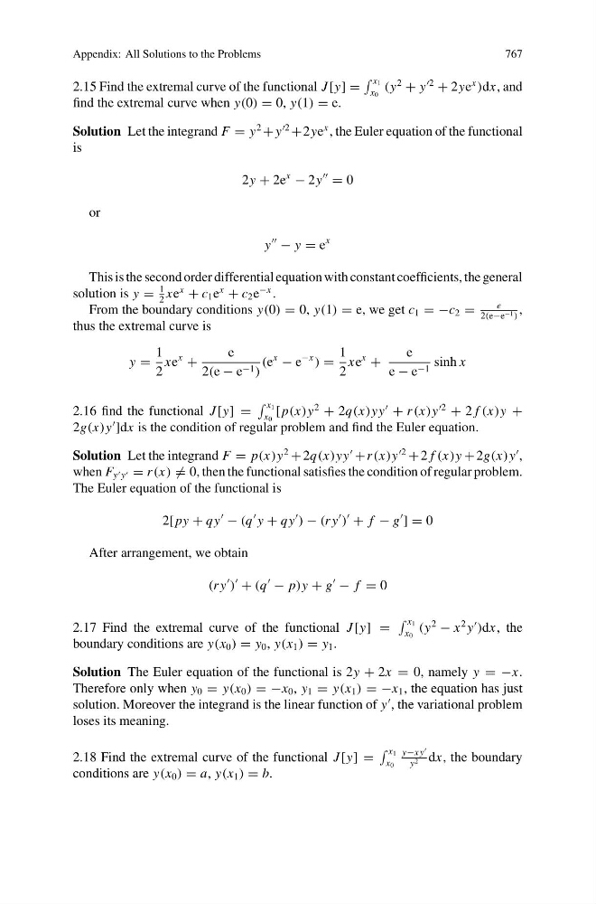
2.15 Find the extremal curve of the functional J [y] =
x 1
x 0
(y
2
+ y
2
+ 2ye
x
)dx, and
find the extremal curve when y(0) = 0, y(1) = e.
Solution Let the integrand F = y
2
+ y
2
+2ye
x , the Euler equation of the functional
is
2y + 2e
x
− 2y
= 0
or
y
− y = e
x
This is the second order differential equation with constant coefficients, the general
solution is y =
1
2
xe
x
+ c 1 e
x
+ c 2 e
−x .
From the boundary conditions y(0) = 0, y(1) = e, we get c 1 = −c 2 =
e
2(e−e −1 )
,
thus the extremal curve is
y =
1
2
xe
x
+
e
2(e − e −1 )
(e
x
− e
−x
) =
1
2
xe
x
+
e
e − e −1 sinh x
2.16 find the functional J [y] =
x 1
x 0
[ p(x)y
2
+ 2q(x)yy
+ r (x)y
2
+ 2 f (x)y +
2g(x)y
]dx is the condition of regular problem and find the Euler equation.
Solution Let the integrand F = p(x)y
2
+ 2q(x)yy
+ r (x)y
2
+ 2 f (x)y + 2g(x)y
,
when F y y = r (x) = 0, then the functional satisfies the condition of regular problem.
The Euler equation of the functional is
2[ py + qy
− (q
y + qy
) − (r y
)
+ f − g
] = 0
After arrangement, we obtain
(r y
)
+ (q
− p)y + g
− f = 0
2.17 Find the extremal curve of the functional J [y] =
x 1
x 0
(y
2
− x
2 y
)dx, the
boundary conditions are y(x 0 ) = y 0 , y(x 1 ) = y 1 .
Solution The Euler equation of the functional is 2y + 2x = 0, namely y = −x.
Therefore only when y 0 = y(x 0 ) = −x 0 , y 1 = y(x 1 ) = −x 1 , the equation has just
solution. Moreover the integrand is the linear function of y
, the variational problem
loses its meaning.
2.18 Find the extremal curve of the functional J [y] =
x 1
x 0
y−xy
y 2 dx, the boundary
conditions are y(x 0 ) = a, y(x 1 ) = b.