

764
Appendix: All Solutions to the Problems
Putting y
= p, then the above equation can be written as
d p
p
+
dx
x
= 0
Integrating, we get
px = y
x = c 1
Integrating again, we get
y = c 1 ln x + c 2
From the boundary conditions y(1) = 0, y(e) = 1, we get c 2 = 0, c 1 = 1, thus
the extremal curve is y = ln x.
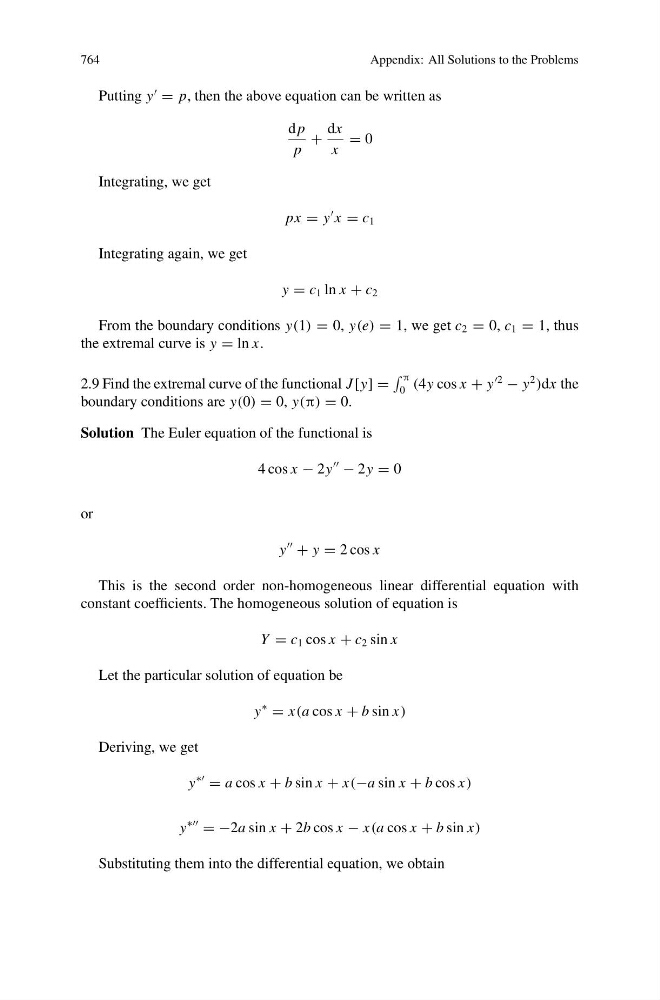
2.9 Find the extremal curve of the functional J [y] =
π
0 (4y cos x + y
2
− y
2
)dx the
boundary conditions are y(0) = 0, y(π) = 0.
Solution The Euler equation of the functional is
4 cos x − 2y
− 2y = 0
or
y
+ y = 2 cos x
This is the second order non-homogeneous linear differential equation with
constant coefficients. The homogeneous solution of equation is
Y = c 1 cos x + c 2 sin x
Let the particular solution of equation be
y
∗
= x(a cos x + b sin x)
Deriving, we get
y
∗∗
= a cos x + b sin x + x(−a sin x + b cos x)
y
∗∗∗
= −2a sin x + 2b cos x − x(a cos x + b sin x)
Substituting them into the differential equation, we obtain