10.7 Variational Problems of Functionals with Series-Type …
717
vector, and for a vector a, there is ∇ · a = a · ∇, make use of the comma convention,
F ,i =
∂ F
∂ x i
= ∂ i F, there is
∇ · ( A n − 1
· D) = ( A n − 1
· D) · ∇ = ∂ i e i · (A j 1 j 2 ··· jn e j 1 e j 2 · · · e jn
n − 1
· D k 1 k 2 ···k n−1 e k 1 e k 2 · · · e k n−1 )
= (A j 1 j 2 ··· jn ,i D k 1 k 2 ···k n−1 + A j 1 j 2 ··· jn D k 1 k 2 ···k n−1 ,i )(e i · e j 1 )(e j 2 · e k n−1 ) · · · (e jn · e k 1 )
= A j 1 j 2 ··· jn ,i D k 1 k 2 ···k n−1 (e i · e j 1 )(e j 2 · e k n−1 ) · · · (e jn · e k 1 )
+ A j 1 j 2 ··· jn D k 1 k 2 ···k n−1 ,i (e i · e j 1 )(e j 2 · e k n−1 ) · · · (e jn · e k 1 )
= (∂ i e i · A j 1 j 2 ··· jn e j 1 e j 2 · · · e jn ) n − 1
· D k 1 k 2 ···k n−1 e k 1 e k 2 · · · e k n−1
+ A j 1 j 2 ··· jn e j 1 e j 2 · · · e jn
n
· D k 1 k 2 ···k n−1 e k 1 e k 2 · · · e k n−1 ∂ i e i
= (∇ · A) n − 1
· D + A n
· D∇ = D n − 1
· (∇ · A) + D∇ n
· A
(10.7.1)
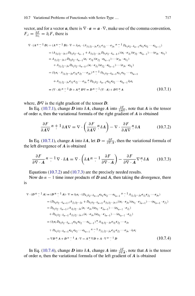
where, D∇ is the right gradient of the tensor D.
In Eq. (10.7.1), change D into δ A, change A into
∂ F
∂ A∇
, note that A is the tensor
of order n, then the variational formula of the right gradient of A is obtained
∂ F
∂ A∇
n + 1
· δ A∇ = ∇ ·
∂ F
∂ A∇
n
· δ A
− ∇ ·
∂ F
∂ A∇
n
· δ A
(10.7.2)
In Eq. (10.7.1), change A into δ A, let D =
∂ F
∂∇· A
, then the variational formula of
the left divergence of A is obtained
∂ F
∂∇ · A
n − 1
· ∇ · δ A = ∇ ·
δ A n − 1
·
∂ F
∂∇ · A
−
∂ F
∂∇ · A
∇ n
· δ A
(10.7.3)
Equations (10.7.2) and (10.7.3) are the precisely needed results.
Now do n − 1 time inner products of D and A, then taking the divergence, there
is
∇ · ( D n − 1
· A) = ( D n − 1
· A) · ∇ = ∂ i e i · (D k 1 k 2 ···k n−1 e k 1 e k 2 · · · e k n−1
n − 1
· A j 1 j 2 ··· jn e j 1 e j 2 · · · e jn )
= (D k 1 k 2 ···k n−1 ,i A j 1 j 2 ··· jn + D k 1 k 2 ···k n−1 A j 1 j 2 ··· jn ,i )(e i · e jn )(e k 1 · e j n−1 ) · · · (e k n−1 · e j 1 )
= D k 1 k 2 ···k n−1 ,i A j 1 j 2 ··· jn (e i · e jn )(e k 1 · e j n−1 ) · · · (e k n−1 · e j 1 )
+ D k 1 k 2 ···k n−1 A j 1 j 2 ··· jn ,i (e i · e jn )(e k 1 · e j n−1 ) · · · (e k n−1 · e j 1 )
= (∂ i e i D k 1 k 2 ···k n−1 e k 1 e k 2 · · · e k n−1 ) n
· A j 1 j 2 ··· jn e j 1 e j 2 · · · e jn
+ D k 1 k 2 ···k n−1 e k 1 e k 2 · · · e k n−1
n − 1
· A j 1 j 2 ··· jn e j 1 e j 2 · · · e jn · ∂ i e i
= ∇ D n
· A + D n − 1
· A · ∇ = A n
· ∇ D + A · ∇ n − 1
· D
(10.7.4)
In Eq. (10.7.4), change D into δ A, change A into
∂ F
∂∇ A
, note that A is the tensor
of order n, then the variational formula of the left gradient of A is obtained