700
10 Variational Problems of Functionals with Vector, Tensor …
Π
∗c
2 [ P, R, u] =
V
[Σ
c2
( J( P · R)) − tr P + u · ( P · ∇ + ρ 0 b)]dV
−
A u
u 1 · P · ndA +
A P
u · ( P · N − P 1N )d A
(1)
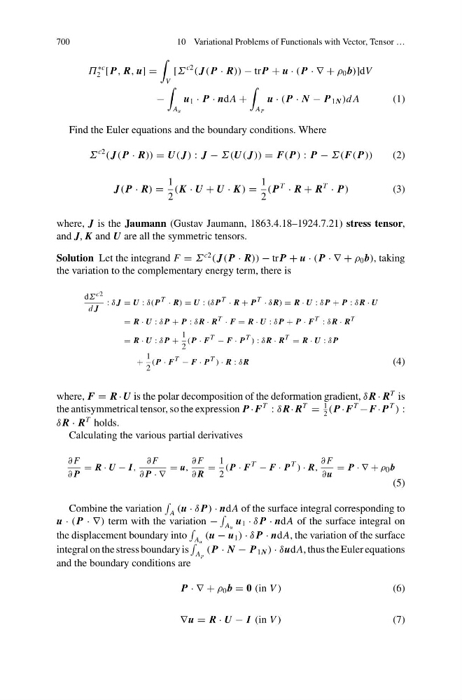
Find the Euler equations and the boundary conditions. Where
Σ
c2
( J( P · R)) = U( J) : J − Σ(U( J)) = F( P) : P − Σ(F( P))
(2)
J( P · R) =
1
2
(K · U + U · K ) =
1
2
( P
T
· R + R
T
· P)
(3)
where, J is the Jaumann (Gustav Jaumann, 1863.4.18–1924.7.21) stress tensor,
and J, K and U are all the symmetric tensors.
Solution Let the integrand F = Σ
c2
( J( P · R)) − tr P + u · ( P · ∇ + ρ 0 b), taking
the variation to the complementary energy term, there is
dΣ c2
d J
: δ J = U : δ( P T · R) = U : (δ P T · R + P T · δ R) = R · U : δ P + P : δ R · U
= R · U : δ P + P : δ R · R T · F = R · U : δ P + P · F T : δ R · R T
= R · U : δ P +
1
2
( P · F T − F · P T ) : δ R · R T = R · U : δ P
+
1
2
( P · F T − F · P T ) · R : δ R
(4)
where, F = R · U is the polar decomposition of the deformation gradient, δ R · R
T is
the antisymmetrical tensor, so the expression P · F
T
: δ R· R
T
=
1
2
( P · F
T
− F· P
T
) :
δ R · R
T holds.
Calculating the various partial derivatives
∂ F
∂ P
= R · U − I,
∂ F
∂ P · ∇
= u,
∂ F
∂ R
=
1
2
( P · F T − F · P T ) · R,
∂ F
∂ u
= P · ∇ + ρ 0 b
(5)
Combine the variation
A (u · δ P) · ndA of the surface integral corresponding to
u · ( P · ∇) term with the variation −
A u
u 1 · δ P · ndA of the surface integral on
the displacement boundary into
A u
(u − u 1 ) · δ P · ndA, the variation of the surface
integral on the stress boundary is
A p
( P · N − P 1N ) · δudA, thus the Euler equations
and the boundary conditions are
P · ∇ + ρ 0 b = 0 (in V )
(6)
∇u = R · U − I (in V )
(7)