10.4 The Euler Equations of Divergence Type Functionals
669
The natural boundary conditions are
∂ F
∂∇ · (ab)
S
= 0
(6)
10.5 The Euler Equations of Rotation Type Functionals
A functional that the variable can finally be represented as the rotation is called the
rotation type functional, or if a function on which a functional is dependent can
finally expressed by the rotation of the function, then such a functional is called the
rotation type functional. The variational problems of the rotation type functional
are discussed in this section.
Example 10.5.1 The functional with the secondary rotation of vector. Let the
functional
J =
V
F(a, ∇ × ∇ × a)dV
(1)
Derive its Euler equation and natural boundary conditions.
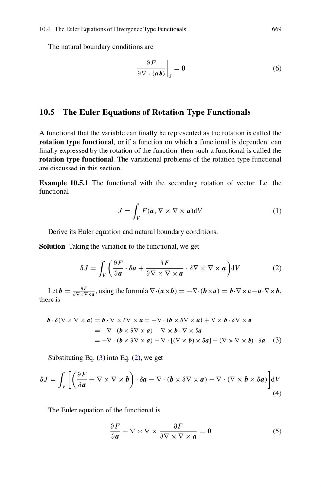
Solution Taking the variation to the functional, we get
δ J =
V
∂ F
∂ a
· δa +
∂ F
∂∇ × ∇ × a
· δ∇ × ∇ × a
dV
(2)
Let b =
∂ F
∂∇×∇×a
, using the formula ∇·(a×b) = −∇·(b×a) = b·∇×a−a·∇×b,
there is
b · δ(∇ × ∇ × a) = b · ∇ × δ∇ × a = −∇ · (b × δ∇ × a) + ∇ × b · δ∇ × a
= −∇ · (b × δ∇ × a) + ∇ × b · ∇ × δa
= −∇ · (b × δ∇ × a) − ∇ · [(∇ × b) × δa] + (∇ × ∇ × b) · δa (3)
Substituting Eq. (3) into Eq. (2), we get
δ J =
V
∂ F
∂ a
+ ∇ × ∇ × b
· δa − ∇ · (b × δ∇ × a) − ∇ · (∇ × b × δa)
dV
(4)
The Euler equation of the functional is
∂ F
∂ a
+ ∇ × ∇ ×
∂ F
∂∇ × ∇ × a
= 0
(5)