638
10 Variational Problems of Functionals with Vector, Tensor …
p + k
2 p + jωρq = 0
The boundary condition is
∇ p · n + jωρv n = 0 or p x n x + p y n y + p z n z = −jωρv n or
∂ p
∂n
= −jωρv n (on S)
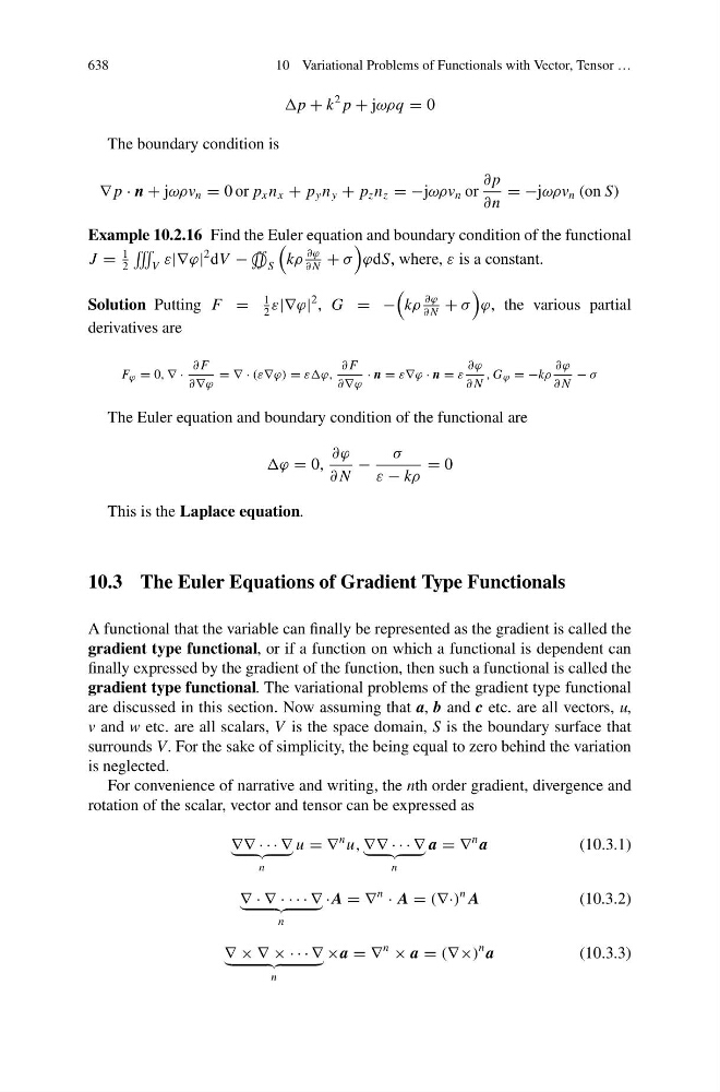
Example 10.2.16 Find the Euler equation and boundary condition of the functional
J =
1
2
˝
V ε|∇ϕ|
2 dV −
S
kρ
∂ϕ
∂ N
+ σ
ϕdS, where, ε is a constant.
Solution Putting F =
1
2
ε|∇ϕ|
2 , G = −
kρ
∂ϕ
∂ N
+ σ
ϕ, the various partial
derivatives are
F ϕ = 0, ∇ ·
∂ F
∂∇ϕ
= ∇ · (ε∇ϕ) = εεϕ,
∂ F
∂∇ϕ
· n = ε∇ϕ · n = ε
∂ϕ
∂ N
, G ϕ = −kρ
∂ϕ
∂ N
− σ
The Euler equation and boundary condition of the functional are
ϕ = 0,
∂ϕ
∂ N
−
σ
ε − kρ
= 0
This is the Laplace equation.
10.3 The Euler Equations of Gradient Type Functionals
A functional that the variable can finally be represented as the gradient is called the
gradient type functional, or if a function on which a functional is dependent can
finally expressed by the gradient of the function, then such a functional is called the
gradient type functional. The variational problems of the gradient type functional
are discussed in this section. Now assuming that a, b and c etc. are all vectors, u,
v and w etc. are all scalars, V is the space domain, S is the boundary surface that
surrounds V. For the sake of simplicity, the being equal to zero behind the variation
is neglected.
For convenience of narrative and writing, the nth order gradient, divergence and
rotation of the scalar, vector and tensor can be expressed as
∇∇ · · · ∇
n
u = ∇
n u, ∇∇ · · · ∇
n
a = ∇
n a
(10.3.1)
∇ · ∇ · · · · ∇
n
· A = ∇
n
· A = (∇·)
n A
(10.3.2)
∇ × ∇ × · · · ∇
n
×a = ∇
n
× a = (∇×)
n a
(10.3.3)