

9.1 Fundamental Conceptions in Mechanics
515
necessarily occur practically. The so-called constraint allowance refers to the virtual
displacement of elastic body must satisfy the deformation compatibility conditions
and geometrical boundary conditions. The constraint conditions here refer to the
relations between the elastic body inside and the relations between the inside and the
outside. The so-called arbitrary infinitesimal displacement refers to that the displacement has nothing to do with the external load state of elastic body, has nothing to
do with the time, meanwhile it is an infinitely small quantity. The virtual displacement is a geometry concept, which has nothing to do with the time progress, is only
determined by the location of particle or particle system and the constraint.
9.1.4 Relations Between Strains and Displacements
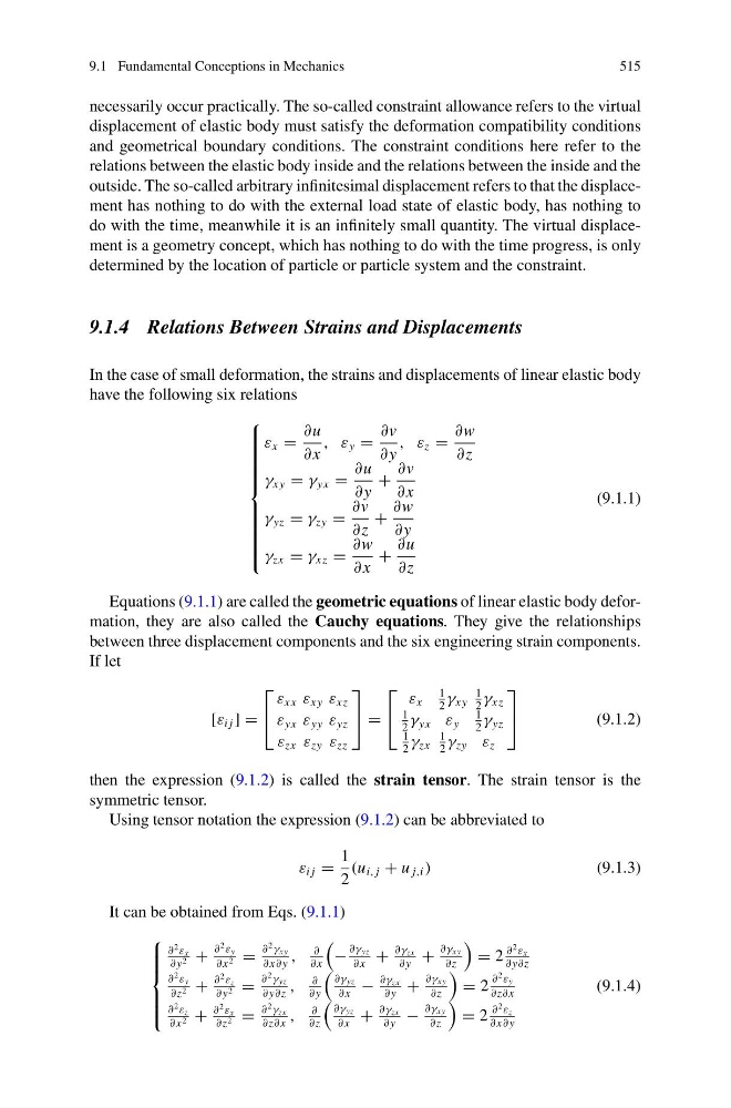
In the case of small deformation, the strains and displacements of linear elastic body
have the following six relations
⎧
⎪ ⎪ ⎪ ⎪ ⎪ ⎪ ⎪ ⎪ ⎪ ⎨
⎪ ⎪ ⎪ ⎪ ⎪ ⎪ ⎪ ⎪ ⎪ ⎩
ε x =
∂u
∂ x
, ε y =
∂v
∂ y
, ε z =
∂w
∂z
γ xy = γ yx =
∂u
∂ y
+
∂v
∂ x
γ yz = γ zy =
∂v
∂z
+
∂w
∂ y
γ zx = γ xz =
∂w
∂ x
+
∂u
∂z
(9.1.1)
Equations (9.1.1) are called the geometric equations of linear elastic body deformation, they are also called the Cauchy equations. They give the relationships
between three displacement components and the six engineering strain components.
If let
[ε i j ] =
⎡
⎣
ε xx ε xy ε xz
ε yx ε yy ε yz
ε zx ε zy ε zz
⎤
⎦ =
⎡
⎣
ε x
1
2
γ xy
1
2
γ xz
1
2
γ yx ε y
1
2
γ yz
1
2
γ zx
1
2
γ zy ε z
⎤
⎦
(9.1.2)
then the expression (9.1.2) is called the strain tensor. The strain tensor is the
symmetric tensor.
Using tensor notation the expression (9.1.2) can be abbreviated to
ε i j =
1
2
(u i, j + u j,i )
(9.1.3)
It can be obtained from Eqs. (9.1.1)
⎧
⎪ ⎪ ⎪ ⎨
⎪ ⎪ ⎪ ⎩
∂
2 ε x
∂ y 2 +
∂
2 ε y
∂ x 2 =
∂
2 γ xy
∂ x∂ y
,
∂
∂ x
−
∂γ yz
∂ x
+
∂γ zx
∂ y
+
∂γ xy
∂z
= 2
∂
2 ε x
∂ y∂z
∂
2 ε y
∂z 2 +
∂
2 ε z
∂ y 2 =
∂
2 γ yz
∂ y∂z
,
∂
∂ y
∂γ yz
∂ x
−
∂γ zx
∂ y
+
∂γ xy
∂z
= 2
∂
2 ε y
∂z∂ x
∂
2 ε z
∂ x 2 +
∂
2 ε x
∂z 2 =
∂
2 γ zx
∂z∂ x
,
∂
∂z
∂γ yz
∂ x
+
∂γ zx
∂ y
−
∂γ xy
∂z
= 2
∂
2 ε z
∂ x∂ y
(9.1.4)
515
necessarily occur practically. The so-called constraint allowance refers to the virtual
displacement of elastic body must satisfy the deformation compatibility conditions
and geometrical boundary conditions. The constraint conditions here refer to the
relations between the elastic body inside and the relations between the inside and the
outside. The so-called arbitrary infinitesimal displacement refers to that the displacement has nothing to do with the external load state of elastic body, has nothing to
do with the time, meanwhile it is an infinitely small quantity. The virtual displacement is a geometry concept, which has nothing to do with the time progress, is only
determined by the location of particle or particle system and the constraint.
9.1.4 Relations Between Strains and Displacements
In the case of small deformation, the strains and displacements of linear elastic body
have the following six relations
⎧
⎪ ⎪ ⎪ ⎪ ⎪ ⎪ ⎪ ⎪ ⎪ ⎨
⎪ ⎪ ⎪ ⎪ ⎪ ⎪ ⎪ ⎪ ⎪ ⎩
ε x =
∂u
∂ x
, ε y =
∂v
∂ y
, ε z =
∂w
∂z
γ xy = γ yx =
∂u
∂ y
+
∂v
∂ x
γ yz = γ zy =
∂v
∂z
+
∂w
∂ y
γ zx = γ xz =
∂w
∂ x
+
∂u
∂z
(9.1.1)
Equations (9.1.1) are called the geometric equations of linear elastic body deformation, they are also called the Cauchy equations. They give the relationships
between three displacement components and the six engineering strain components.
If let
[ε i j ] =
⎡
⎣
ε xx ε xy ε xz
ε yx ε yy ε yz
ε zx ε zy ε zz
⎤
⎦ =
⎡
⎣
ε x
1
2
γ xy
1
2
γ xz
1
2
γ yx ε y
1
2
γ yz
1
2
γ zx
1
2
γ zy ε z
⎤
⎦
(9.1.2)
then the expression (9.1.2) is called the strain tensor. The strain tensor is the
symmetric tensor.
Using tensor notation the expression (9.1.2) can be abbreviated to
ε i j =
1
2
(u i, j + u j,i )
(9.1.3)
It can be obtained from Eqs. (9.1.1)
⎧
⎪ ⎪ ⎪ ⎨
⎪ ⎪ ⎪ ⎩
∂
2 ε x
∂ y 2 +
∂
2 ε y
∂ x 2 =
∂
2 γ xy
∂ x∂ y
,
∂
∂ x
−
∂γ yz
∂ x
+
∂γ zx
∂ y
+
∂γ xy
∂z
= 2
∂
2 ε x
∂ y∂z
∂
2 ε y
∂z 2 +
∂
2 ε z
∂ y 2 =
∂
2 γ yz
∂ y∂z
,
∂
∂ y
∂γ yz
∂ x
−
∂γ zx
∂ y
+
∂γ xy
∂z
= 2
∂
2 ε y
∂z∂ x
∂
2 ε z
∂ x 2 +
∂
2 ε x
∂z 2 =
∂
2 γ zx
∂z∂ x
,
∂
∂z
∂γ yz
∂ x
+
∂γ zx
∂ y
−
∂γ xy
∂z
= 2
∂
2 ε z
∂ x∂ y
(9.1.4)