

8.8 Introduction to the Famous Scientists
507
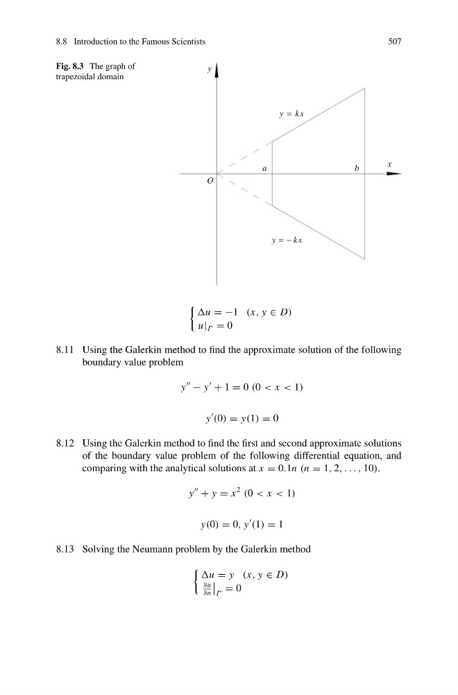
Fig. 8.3 The graph of
trapezoidal domain
O
x
y
a
b
y = kx
y = − kx
u = −1 (x, y ∈ D)
u| Γ = 0
8.11 Using the Galerkin method to find the approximate solution of the following
boundary value problem
y
− y
+ 1 = 0 (0 < x < 1)
y
(0) = y(1) = 0
8.12 Using the Galerkin method to find the first and second approximate solutions
of the boundary value problem of the following differential equation, and
comparing with the analytical solutions at x = 0.1n (n = 1, 2, . . . , 10).
y
+ y = x
2
(0 < x < 1)
y(0) = 0, y
(1) = 1
8.13 Solving the Neumann problem by the Galerkin method
u = y (x, y ∈ D)
∂u
∂n
Γ = 0
507
Fig. 8.3 The graph of
trapezoidal domain
O
x
y
a
b
y = kx
y = − kx
u = −1 (x, y ∈ D)
u| Γ = 0
8.11 Using the Galerkin method to find the approximate solution of the following
boundary value problem
y
− y
+ 1 = 0 (0 < x < 1)
y
(0) = y(1) = 0
8.12 Using the Galerkin method to find the first and second approximate solutions
of the boundary value problem of the following differential equation, and
comparing with the analytical solutions at x = 0.1n (n = 1, 2, . . . , 10).
y
+ y = x
2
(0 < x < 1)
y(0) = 0, y
(1) = 1
8.13 Solving the Neumann problem by the Galerkin method
u = y (x, y ∈ D)
∂u
∂n
Γ = 0