

502
8 Direct Methods of Variational Problems
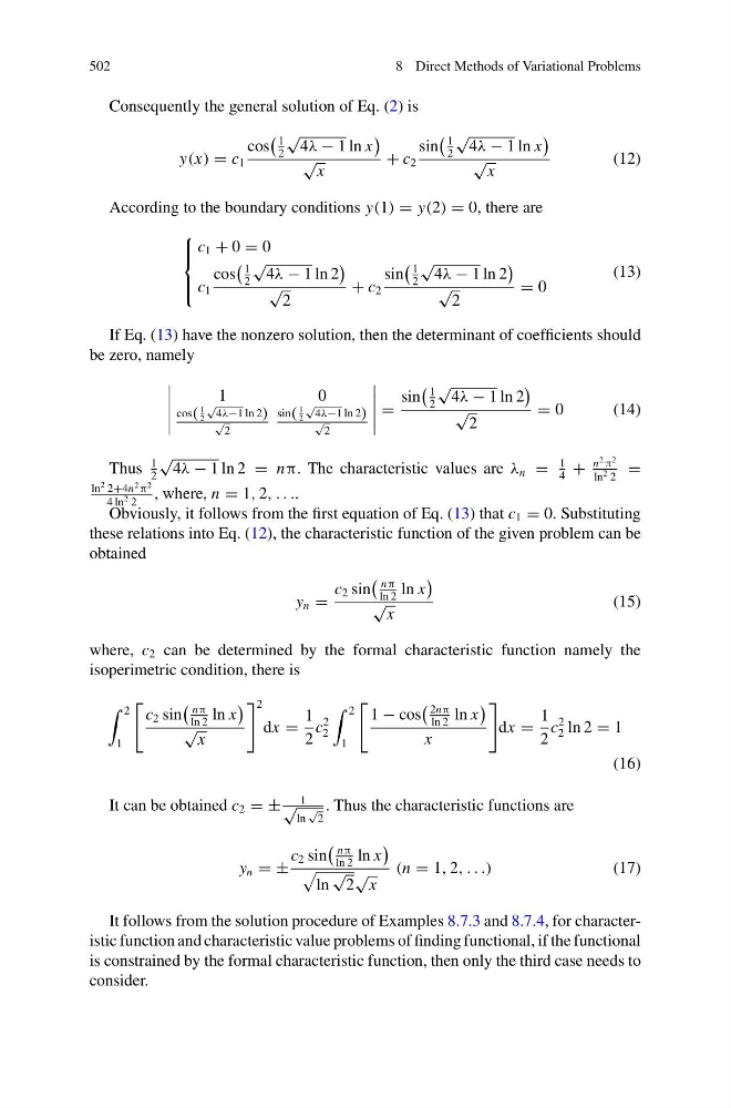
Consequently the general solution of Eq. (2) is
y(x) = c 1
cos
1
2
√
4λ − 1 ln x
√
x
+ c 2
sin
1
2
√
4λ − 1 ln x
√
x
(12)
According to the boundary conditions y(1) = y(2) = 0, there are
⎧
⎪ ⎨
⎪ ⎩
c 1 + 0 = 0
c 1
cos
1
2
√
4λ − 1 ln 2
√
2
+ c 2
sin
1
2
√
4λ − 1 ln 2
√
2
= 0
(13)
If Eq. (13) have the nonzero solution, then the determinant of coefficients should
be zero, namely
1
0
cos(
1
2
√
4λ−1 ln 2)
√
2
sin(
1
2
√
4λ−1 ln 2)
√
2
=
sin
1
2
√
4λ − 1 ln 2
√
2
= 0
( 1 4 )
Thus
1
2
√
4λ − 1 ln 2 = nπ. The characteristic values are λ n =
1
4
+
n
2 π
2
ln
2 2
=
ln
2 2+4n
2 π
2
4 ln
2 2
, where, n = 1, 2, . . ..
Obviously, it follows from the first equation of Eq. (13) that c 1 = 0. Substituting
these relations into Eq. (12), the characteristic function of the given problem can be
obtained
y n =
c 2 sin
nπ
ln 2
ln x
√
x
(15)
where, c 2 can be determined by the formal characteristic function namely the
isoperimetric condition, there is
2
1
c 2 sin
nπ
ln 2
ln x
√
x
2
dx =
1
2
c
2
2
2
1
1 − cos
2nπ
ln 2
ln x
x
dx =
1
2
c
2
2 ln 2 = 1
(16)
It can be obtained c 2 = ±
1
√
ln
√
2
. Thus the characteristic functions are
y n = ±
c 2 sin
nπ
ln 2
ln x
ln
√
2
√
x
(n = 1, 2, . . .)
(17)
It follows from the solution procedure of Examples 8.7.3 and 8.7.4, for characteristic function and characteristic value problems of finding functional, if the functional
is constrained by the formal characteristic function, then only the third case needs to
consider.
8 Direct Methods of Variational Problems
Consequently the general solution of Eq. (2) is
y(x) = c 1
cos
1
2
√
4λ − 1 ln x
√
x
+ c 2
sin
1
2
√
4λ − 1 ln x
√
x
(12)
According to the boundary conditions y(1) = y(2) = 0, there are
⎧
⎪ ⎨
⎪ ⎩
c 1 + 0 = 0
c 1
cos
1
2
√
4λ − 1 ln 2
√
2
+ c 2
sin
1
2
√
4λ − 1 ln 2
√
2
= 0
(13)
If Eq. (13) have the nonzero solution, then the determinant of coefficients should
be zero, namely
1
0
cos(
1
2
√
4λ−1 ln 2)
√
2
sin(
1
2
√
4λ−1 ln 2)
√
2
=
sin
1
2
√
4λ − 1 ln 2
√
2
= 0
( 1 4 )
Thus
1
2
√
4λ − 1 ln 2 = nπ. The characteristic values are λ n =
1
4
+
n
2 π
2
ln
2 2
=
ln
2 2+4n
2 π
2
4 ln
2 2
, where, n = 1, 2, . . ..
Obviously, it follows from the first equation of Eq. (13) that c 1 = 0. Substituting
these relations into Eq. (12), the characteristic function of the given problem can be
obtained
y n =
c 2 sin
nπ
ln 2
ln x
√
x
(15)
where, c 2 can be determined by the formal characteristic function namely the
isoperimetric condition, there is
2
1
c 2 sin
nπ
ln 2
ln x
√
x
2
dx =
1
2
c
2
2
2
1
1 − cos
2nπ
ln 2
ln x
x
dx =
1
2
c
2
2 ln 2 = 1
(16)
It can be obtained c 2 = ±
1
√
ln
√
2
. Thus the characteristic functions are
y n = ±
c 2 sin
nπ
ln 2
ln x
ln
√
2
√
x
(n = 1, 2, . . .)
(17)
It follows from the solution procedure of Examples 8.7.3 and 8.7.4, for characteristic function and characteristic value problems of finding functional, if the functional
is constrained by the formal characteristic function, then only the third case needs to
consider.