

498
8 Direct Methods of Variational Problems
⎧
⎪ ⎪ ⎪ ⎨
⎪ ⎪ ⎪ ⎩
1
2
+
π
2
8
− λa
2
1
2
−
2
π 2
a 1 +
λ
2a
2
π 2 −
3
2
a 2 = 0
λ
2a
2
π 2 −
3
2
a 1 +
9π
2
8
+
1
2
− λa
2
1
2
−
2
9π 2
a 2 = 0
(17)
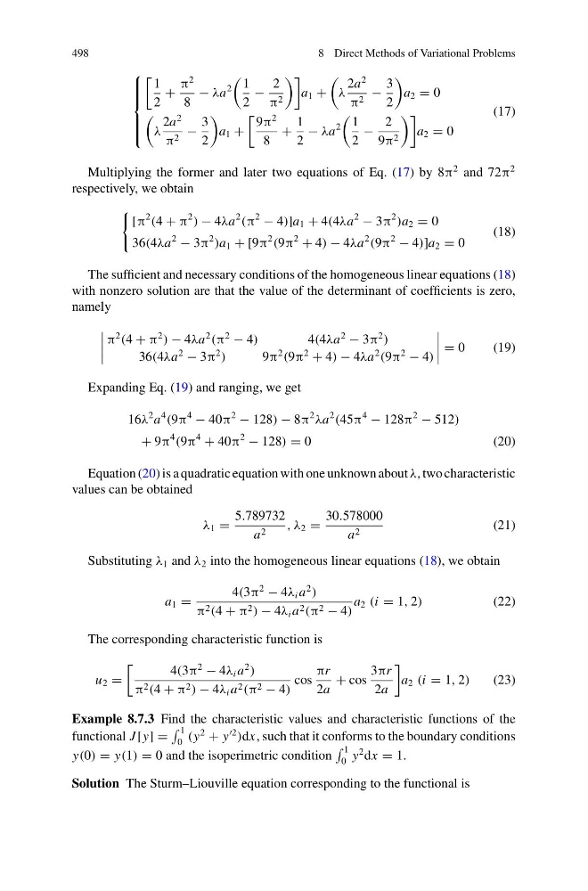
Multiplying the former and later two equations of Eq. (17) by 8π
2 and 72π
2
respectively, we obtain
[π
2
(4 + π
2
) − 4λa
2
(π
2
− 4)]a 1 + 4(4λa
2
− 3π
2
)a 2 = 0
36(4λa
2
− 3π
2
)a 1 + [9π
2
(9π
2
+ 4) − 4λa
2
(9π
2
− 4)]a 2 = 0
(18)
The sufficient and necessary conditions of the homogeneous linear equations (18)
with nonzero solution are that the value of the determinant of coefficients is zero,
namely
π
2
(4 + π
2
) − 4λa
2
(π
2
− 4)
4(4λa
2
− 3π
2
)
36(4λa
2
− 3π
2
)
9π
2
(9π
2
+ 4) − 4λa
2
(9π
2
− 4)
= 0
(19)
Expanding Eq. (19) and ranging, we get
16λ
2 a
4
(9π
4
− 40π
2
− 128) − 8π
2
λa
2
(45π
4
− 128π
2
− 512)
+ 9π
4
(9π
4
+ 40π
2
− 128) = 0
( 2 0 )
Equation (20) is a quadratic equation with one unknown about λ, two characteristic
values can be obtained
λ 1 =
5.789732
a 2
, λ 2 =
30.578000
a 2
(21)
Substituting λ 1 and λ 2 into the homogeneous linear equations (18), we obtain
a 1 =
4(3π
2
− 4λ i a
2
)
π 2 (4 + π 2 ) − 4λ i a 2 (π 2 − 4)
a 2 (i = 1, 2)
(22)
The corresponding characteristic function is
u 2 =
4(3π
2
− 4λ i a
2
)
π 2 (4 + π 2 ) − 4λ i a 2 (π 2 − 4)
cos
πr
2a
+ cos
3πr
2a
a 2 (i = 1, 2)
(23)
Example 8.7.3 Find the characteristic values and characteristic functions of the
functional J [y] =
1
0 (y
2
+ y
2
)dx, such that it conforms to the boundary conditions
y(0) = y(1) = 0 and the isoperimetric condition
1
0 y
2 dx = 1.
Solution The Sturm–Liouville equation corresponding to the functional is
8 Direct Methods of Variational Problems
⎧
⎪ ⎪ ⎪ ⎨
⎪ ⎪ ⎪ ⎩
1
2
+
π
2
8
− λa
2
1
2
−
2
π 2
a 1 +
λ
2a
2
π 2 −
3
2
a 2 = 0
λ
2a
2
π 2 −
3
2
a 1 +
9π
2
8
+
1
2
− λa
2
1
2
−
2
9π 2
a 2 = 0
(17)
Multiplying the former and later two equations of Eq. (17) by 8π
2 and 72π
2
respectively, we obtain
[π
2
(4 + π
2
) − 4λa
2
(π
2
− 4)]a 1 + 4(4λa
2
− 3π
2
)a 2 = 0
36(4λa
2
− 3π
2
)a 1 + [9π
2
(9π
2
+ 4) − 4λa
2
(9π
2
− 4)]a 2 = 0
(18)
The sufficient and necessary conditions of the homogeneous linear equations (18)
with nonzero solution are that the value of the determinant of coefficients is zero,
namely
π
2
(4 + π
2
) − 4λa
2
(π
2
− 4)
4(4λa
2
− 3π
2
)
36(4λa
2
− 3π
2
)
9π
2
(9π
2
+ 4) − 4λa
2
(9π
2
− 4)
= 0
(19)
Expanding Eq. (19) and ranging, we get
16λ
2 a
4
(9π
4
− 40π
2
− 128) − 8π
2
λa
2
(45π
4
− 128π
2
− 512)
+ 9π
4
(9π
4
+ 40π
2
− 128) = 0
( 2 0 )
Equation (20) is a quadratic equation with one unknown about λ, two characteristic
values can be obtained
λ 1 =
5.789732
a 2
, λ 2 =
30.578000
a 2
(21)
Substituting λ 1 and λ 2 into the homogeneous linear equations (18), we obtain
a 1 =
4(3π
2
− 4λ i a
2
)
π 2 (4 + π 2 ) − 4λ i a 2 (π 2 − 4)
a 2 (i = 1, 2)
(22)
The corresponding characteristic function is
u 2 =
4(3π
2
− 4λ i a
2
)
π 2 (4 + π 2 ) − 4λ i a 2 (π 2 − 4)
cos
πr
2a
+ cos
3πr
2a
a 2 (i = 1, 2)
(23)
Example 8.7.3 Find the characteristic values and characteristic functions of the
functional J [y] =
1
0 (y
2
+ y
2
)dx, such that it conforms to the boundary conditions
y(0) = y(1) = 0 and the isoperimetric condition
1
0 y
2 dx = 1.
Solution The Sturm–Liouville equation corresponding to the functional is