

482
8 Direct Methods of Variational Problems
+ a
9 b
7 64
105
×
128
105
a 1 + a
11 b
5 64
105
×
128
5 × 33
a 1 + a
9 b
9 64
105
×
128
35
a 2 +
a
11 b
7 64
105
×
128 × 2
35 × 33
a 2 + a
13 b
5 64
105
×
128
5 × 143
a 2
+
64
105
×
128 × 4
105 × 11
(a
11 b
7
+ a
7 b
11
)a 2 −
64
105
×
1
15
(a
7 b
5
+ a
5 b
7
)m = 0
Simplifying, we get
[77(a
4
+ b
4
) + 44a
2 b
2
]a 1 + 11(a
2 b
4
+ a
4 b
2
)a 2 + 7(a
6
+ b
6
)a 2 =
539
128
m
143(a
2 b
4
+ a
4 b
2
)a 1 + 91(b
6
+ a
6
)a 1 + 858a
4 b
4 a 2
+ 78(a
2 b
6
+ a
6 b
2
)a 2 + 21(b
8
+ a
8
)a 2 =
1001
128
(a
2
+ b
2
)m
Solve for a 1 , a 2
a 1 =
154[715a 4 b 4 + 39(a 2 b 6 + a 6 b 2 ) + 7(b 8 + a 8 )]m
128[16885(a 8 b 4 + a 4 b 8 ) + 1232(a 10 b 2 + a 2 b 10 ) + 245(a 12 + b 12 ) + 11336a 6 b 6 ]
(1)
a 2 =
1001[7(a 6 + b 6 ) + 11(a 4 b 2 + a 2 b 4 )]m
128[16885(a 8 b 4 + a 4 b 8 ) + 1232(a 10 b 2 + a 2 b 10 ) + 245(a 12 + b 12 ) + 11336a 6 b 6 ]
(2)
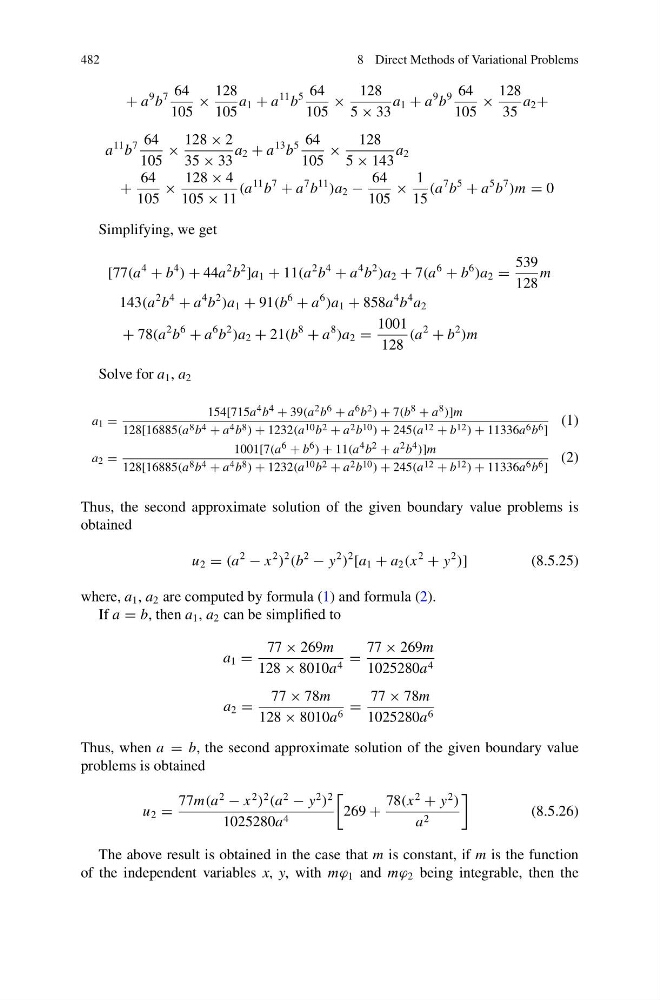
Thus, the second approximate solution of the given boundary value problems is
obtained
u 2 = (a
2
− x
2
)
2
(b
2
− y
2
)
2
[a 1 + a 2 (x
2
+ y
2
)]
(8.5.25)
where, a 1 , a 2 are computed by formula (1) and formula (2).
If a = b, then a 1 , a 2 can be simplified to
a 1 =
77 × 269m
128 × 8010a 4 =
77 × 269m
1025280a 4
a 2 =
77 × 78m
128 × 8010a 6 =
77 × 78m
1025280a 6
Thus, when a = b, the second approximate solution of the given boundary value
problems is obtained
u 2 =
77m(a
2
− x
2
)
2
(a
2
− y
2
)
2
1025280a 4
269 +
78(x
2
+ y
2
)
a 2
(8.5.26)
The above result is obtained in the case that m is constant, if m is the function
of the independent variables x, y, with mϕ 1 and mϕ 2 being integrable, then the
8 Direct Methods of Variational Problems
+ a
9 b
7 64
105
×
128
105
a 1 + a
11 b
5 64
105
×
128
5 × 33
a 1 + a
9 b
9 64
105
×
128
35
a 2 +
a
11 b
7 64
105
×
128 × 2
35 × 33
a 2 + a
13 b
5 64
105
×
128
5 × 143
a 2
+
64
105
×
128 × 4
105 × 11
(a
11 b
7
+ a
7 b
11
)a 2 −
64
105
×
1
15
(a
7 b
5
+ a
5 b
7
)m = 0
Simplifying, we get
[77(a
4
+ b
4
) + 44a
2 b
2
]a 1 + 11(a
2 b
4
+ a
4 b
2
)a 2 + 7(a
6
+ b
6
)a 2 =
539
128
m
143(a
2 b
4
+ a
4 b
2
)a 1 + 91(b
6
+ a
6
)a 1 + 858a
4 b
4 a 2
+ 78(a
2 b
6
+ a
6 b
2
)a 2 + 21(b
8
+ a
8
)a 2 =
1001
128
(a
2
+ b
2
)m
Solve for a 1 , a 2
a 1 =
154[715a 4 b 4 + 39(a 2 b 6 + a 6 b 2 ) + 7(b 8 + a 8 )]m
128[16885(a 8 b 4 + a 4 b 8 ) + 1232(a 10 b 2 + a 2 b 10 ) + 245(a 12 + b 12 ) + 11336a 6 b 6 ]
(1)
a 2 =
1001[7(a 6 + b 6 ) + 11(a 4 b 2 + a 2 b 4 )]m
128[16885(a 8 b 4 + a 4 b 8 ) + 1232(a 10 b 2 + a 2 b 10 ) + 245(a 12 + b 12 ) + 11336a 6 b 6 ]
(2)
Thus, the second approximate solution of the given boundary value problems is
obtained
u 2 = (a
2
− x
2
)
2
(b
2
− y
2
)
2
[a 1 + a 2 (x
2
+ y
2
)]
(8.5.25)
where, a 1 , a 2 are computed by formula (1) and formula (2).
If a = b, then a 1 , a 2 can be simplified to
a 1 =
77 × 269m
128 × 8010a 4 =
77 × 269m
1025280a 4
a 2 =
77 × 78m
128 × 8010a 6 =
77 × 78m
1025280a 6
Thus, when a = b, the second approximate solution of the given boundary value
problems is obtained
u 2 =
77m(a
2
− x
2
)
2
(a
2
− y
2
)
2
1025280a 4
269 +
78(x
2
+ y
2
)
a 2
(8.5.26)
The above result is obtained in the case that m is constant, if m is the function
of the independent variables x, y, with mϕ 1 and mϕ 2 being integrable, then the