

7.8 Variational Problems of Equivalence with Boundary Value Problem …
433
=
Γ 1
p
∂u 1
∂n
u 1 dΓ +
Γ 2
p
∂u 1
∂n
wdΓ +
Γ 2
p
∂u 1
∂n
+ σ u 1
udΓ
=
Γ 1
p
∂u 1
∂n
u 1 dΓ +
Γ 2
kudΓ
(7.8.17)
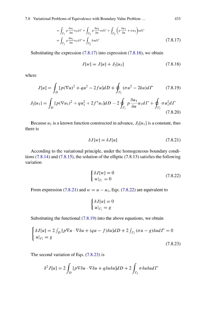
Substituting the expression (7.8.17) into expression (7.8.16), we obtain
J [w] = J [u] + J 2 [u 1 ]
(7.8.18)
where
J [u] =
D
[ p(∇u)
2
+ qu
2
− 2 f u]d D +
Γ 2
(σ u
2
− 2ku)dΓ
(7.8.19)
J 2 [u 1 ] =
D
[ p(∇u 1 )
2
+ qu
2
1 + 2 f
∗ u 1 ]d D − 2
Γ 1
p
∂u 1
∂n
u 1 dΓ +
Γ 2
σ u
2
1 dΓ
(7.8.20)
Because u 1 is a known function constructed in advance, J 2 [u 1 ] is a constant, thus
there is
δ J [w] = δ J [u]
(7.8.21)
According to the variational principle, under the homogeneous boundary conditions (7.8.14) and (7.8.15), the solution of the elliptic (7.8.13) satisfies the following
variation
δ J [w] = 0
w| Γ 1 = 0
(7.8.22)
From expression (7.8.21) and w = u − u 1 , Eqs. (7.8.22) are equivalent to
δ J [u] = 0
u| Γ 1 = g
Substituting the functional (7.8.19) into the above equations, we obtain
δ J [u] = 2
D [ p∇u · ∇δu + (qu − f )δu]d D + 2
Γ 2
(σ u − g)δudΓ = 0
u| Γ 1 = g
(7.8.23)
The second variation of Eqs. (7.8.23) is
δ
2 J [u] = 2
D
[ p∇δu · ∇δu + qδuδu]d D + 2
Γ 2
σ δuδudΓ
433
=
Γ 1
p
∂u 1
∂n
u 1 dΓ +
Γ 2
p
∂u 1
∂n
wdΓ +
Γ 2
p
∂u 1
∂n
+ σ u 1
udΓ
=
Γ 1
p
∂u 1
∂n
u 1 dΓ +
Γ 2
kudΓ
(7.8.17)
Substituting the expression (7.8.17) into expression (7.8.16), we obtain
J [w] = J [u] + J 2 [u 1 ]
(7.8.18)
where
J [u] =
D
[ p(∇u)
2
+ qu
2
− 2 f u]d D +
Γ 2
(σ u
2
− 2ku)dΓ
(7.8.19)
J 2 [u 1 ] =
D
[ p(∇u 1 )
2
+ qu
2
1 + 2 f
∗ u 1 ]d D − 2
Γ 1
p
∂u 1
∂n
u 1 dΓ +
Γ 2
σ u
2
1 dΓ
(7.8.20)
Because u 1 is a known function constructed in advance, J 2 [u 1 ] is a constant, thus
there is
δ J [w] = δ J [u]
(7.8.21)
According to the variational principle, under the homogeneous boundary conditions (7.8.14) and (7.8.15), the solution of the elliptic (7.8.13) satisfies the following
variation
δ J [w] = 0
w| Γ 1 = 0
(7.8.22)
From expression (7.8.21) and w = u − u 1 , Eqs. (7.8.22) are equivalent to
δ J [u] = 0
u| Γ 1 = g
Substituting the functional (7.8.19) into the above equations, we obtain
δ J [u] = 2
D [ p∇u · ∇δu + (qu − f )δu]d D + 2
Γ 2
(σ u − g)δudΓ = 0
u| Γ 1 = g
(7.8.23)
The second variation of Eqs. (7.8.23) is
δ
2 J [u] = 2
D
[ p∇δu · ∇δu + qδuδu]d D + 2
Γ 2
σ δuδudΓ