

5.3 Isoperimetric Problems
337
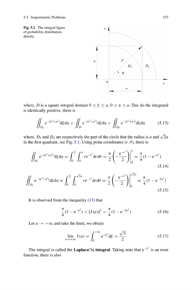
Fig. 5.1 The integral figure
of probability distribution
density
a
a
y
0
x
D 1
D 2
θ
Γ
where, D is a square integral domain 0 ≤ ξ ≤ a, 0 ≤ η ≤ a. Due do the integrand
is identically positive, there is
¨
D 1
e
−(ξ
2 +η
2 ) dξ dη <
¨
D
e
−(ξ
2 +η
2 ) dξ dη <
¨
D 2
e
−(ξ
2 +η
2 ) dξ dη
(5.13)
where, D 1 and D 2 are respectively the part of the circle that the radius is a and
√
2a
in the first quadrant, see Fig. 5.1. Using polar coordinates (r, θ), there is
¨
D 1
e
−(ξ
2 +η
2 ) dξ dη =
π
2
0
a
0
r e
−r
2 dr dθ =
π
2
−
e
−r
2
2
a
0
=
π
4
(1 − e
−a
2 )
(5.14)
¨
D 2
e
−(ξ
2 +η
2 ) dξ dη =
π
2
0
√
2a
0
r e
−r
2 dr dθ =
π
2
−
e
−r
2
2
√
2a
0
=
π
4
(1 − e
−2a
2 )
(5.15)
It is observed from the inequality (13) that
π
4
(1 − e
−a
2 ) < [I (a)]
2
<
π
4
(1 − e
−2a
2 )
(5.16)
Let a → +∞ and take the limit, we obtain
lim
a→+∞
I (a) =
+∞
0
e
−ξ
2 dξ =
√ π
2
(5.17)
The integral is called the Laplace(’s) integral. Taking note that e
−ξ
2 is an even
function, there is also
337
Fig. 5.1 The integral figure
of probability distribution
density
a
a
y
0
x
D 1
D 2
θ
Γ
where, D is a square integral domain 0 ≤ ξ ≤ a, 0 ≤ η ≤ a. Due do the integrand
is identically positive, there is
¨
D 1
e
−(ξ
2 +η
2 ) dξ dη <
¨
D
e
−(ξ
2 +η
2 ) dξ dη <
¨
D 2
e
−(ξ
2 +η
2 ) dξ dη
(5.13)
where, D 1 and D 2 are respectively the part of the circle that the radius is a and
√
2a
in the first quadrant, see Fig. 5.1. Using polar coordinates (r, θ), there is
¨
D 1
e
−(ξ
2 +η
2 ) dξ dη =
π
2
0
a
0
r e
−r
2 dr dθ =
π
2
−
e
−r
2
2
a
0
=
π
4
(1 − e
−a
2 )
(5.14)
¨
D 2
e
−(ξ
2 +η
2 ) dξ dη =
π
2
0
√
2a
0
r e
−r
2 dr dθ =
π
2
−
e
−r
2
2
√
2a
0
=
π
4
(1 − e
−2a
2 )
(5.15)
It is observed from the inequality (13) that
π
4
(1 − e
−a
2 ) < [I (a)]
2
<
π
4
(1 − e
−2a
2 )
(5.16)
Let a → +∞ and take the limit, we obtain
lim
a→+∞
I (a) =
+∞
0
e
−ξ
2 dξ =
√ π
2
(5.17)
The integral is called the Laplace(’s) integral. Taking note that e
−ξ
2 is an even
function, there is also