

5.2 Variational Problems with Differential Constraints
327
∂ F
∂ y j
−
d
dx
∂ F
∂ y
j
+
m
i=1
λ i (x)
∂ϕ i
∂ y
j
+
m
i=1
λ i (x)
∂ϕ i
∂ y j
= 0 ( j = 1, 2, . . . , n) (5.2.6)
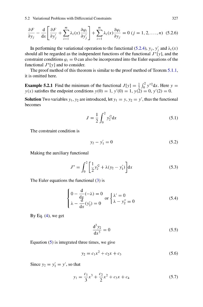
In performing the variational operation to the functional (5.2.4), y j , y
j and λ i (x)
should all be regarded as the independent functions of the functional J
∗
[y], and the
constraint conditions ϕ i = 0 can also be incorporated into the Euler equations of the
functional J
∗
[y] and to consider.
The proof method of this theorem is similar to the proof method of Teorem 5.1.1,
it is omitted here.
Example 5.2.1 Find the minimum of the functional J [y] =
1
2
2
0 y
2 dx. Here y =
y(x) satisfies the endpoint conditions y(0) = 1, y
(0) = 1, y(2) = 0, y
(2) = 0.
Solution Two variables y 1 , y 2 are introduced, let y 1 = y, y 2 = y
, thus the functional
becomes
J =
1
2
2
0
y
2
2 dx
(5.1)
The constraint condition is
y 2 − y
1 = 0
( 5 . 2 )
Making the auxiliary functional
J
∗
=
2
0
1
2
y
2
2 + λ(y 2 − y
1 )
dx
(5.3)
The Euler equations the functional (3) is
⎧
⎪ ⎨
⎪ ⎩
0 −
d
dx
(−λ) = 0
λ −
d
dx
(y
2 ) = 0
or
λ
= 0
λ − y
2 = 0
(5.4)
By Eq. (4), we get
d
3 y 2
dx 3 = 0
(5.5)
Equation (5) is integrated three times, we give
y 2 = c 1 x
2
+ c 2 x + c 3
(5.6)
Since y 2 = y
1 = y
, so that
y 1 =
c 1
3
x
3
+
c 2
2
x
2
+ c 3 x + c 4
(5.7)
327
∂ F
∂ y j
−
d
dx
∂ F
∂ y
j
+
m
i=1
λ i (x)
∂ϕ i
∂ y
j
+
m
i=1
λ i (x)
∂ϕ i
∂ y j
= 0 ( j = 1, 2, . . . , n) (5.2.6)
In performing the variational operation to the functional (5.2.4), y j , y
j and λ i (x)
should all be regarded as the independent functions of the functional J
∗
[y], and the
constraint conditions ϕ i = 0 can also be incorporated into the Euler equations of the
functional J
∗
[y] and to consider.
The proof method of this theorem is similar to the proof method of Teorem 5.1.1,
it is omitted here.
Example 5.2.1 Find the minimum of the functional J [y] =
1
2
2
0 y
2 dx. Here y =
y(x) satisfies the endpoint conditions y(0) = 1, y
(0) = 1, y(2) = 0, y
(2) = 0.
Solution Two variables y 1 , y 2 are introduced, let y 1 = y, y 2 = y
, thus the functional
becomes
J =
1
2
2
0
y
2
2 dx
(5.1)
The constraint condition is
y 2 − y
1 = 0
( 5 . 2 )
Making the auxiliary functional
J
∗
=
2
0
1
2
y
2
2 + λ(y 2 − y
1 )
dx
(5.3)
The Euler equations the functional (3) is
⎧
⎪ ⎨
⎪ ⎩
0 −
d
dx
(−λ) = 0
λ −
d
dx
(y
2 ) = 0
or
λ
= 0
λ − y
2 = 0
(5.4)
By Eq. (4), we get
d
3 y 2
dx 3 = 0
(5.5)
Equation (5) is integrated three times, we give
y 2 = c 1 x
2
+ c 2 x + c 3
(5.6)
Since y 2 = y
1 = y
, so that
y 1 =
c 1
3
x
3
+
c 2
2
x
2
+ c 3 x + c 4
(5.7)