

4.6 One-Sided Variational Problems
309
y =
⎧
⎪ ⎪ ⎪ ⎪ ⎪ ⎪ ⎪ ⎪ ⎨
⎪ ⎪ ⎪ ⎪ ⎪ ⎪ ⎪ ⎪ ⎩
±
R
(x 0 − a) 2 − R 2
R 2 + 2ax 0 − a 2 − x
2
0
(x − x 0 )
x 0 ≤ x ≤
R
2
+ ax 0 − a
2
x 0 − a
±
R 2 − (x − a) 2
R
2
+ ax 0 − a
2
x 0 − a
≤ x ≤
R
2
+ ax 1 − a
2
x 1 − a
∓
R
(x 1 − a) 2 − R 2
R 2 + 2ax 1 − a 2 − x
2
1
(x − x 1 )
R
2
+ ax 1 − a
2
x 1 − a
≤ x ≤ x 1
(8)
When a = 13, R = 5, x 0 = 0 and x 1 = 26, on the left side of the circle, c 1 = ±
5
12
is given, at the moment the tangential point of the extremal curve and the circle is
144
13
, ±
60
13
; On the right side of the circle, c 1 = ∓
5
12
is given, at the moment the
tangential point of the extremal curve and the circle is
194
13
, ±
60
13
. The extremal
curve to be found is
y =
⎧
⎪ ⎪ ⎪ ⎪ ⎪ ⎪ ⎪ ⎨
⎪ ⎪ ⎪ ⎪ ⎪ ⎪ ⎪ ⎩
±
5
12
x
0 ≤ x ≤
144
13
±
25 − (x − 13) 2
144
13
≤ x ≤
194
13
∓
5
12
(x − 26)
194
13
≤ x ≤ 26
(9)
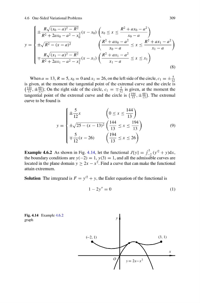
Example 4.6.2 As shown in Fig. 4.14, let the functional J [y] =
3
−2 (y
+ y)dx,
the boundary conditions are y(−2) = 1, y(3) = 1, and all the admissible curves are
located in the plane domain y ≥ 2x − x
2 . Find a curve that can make the functional
attain extremum.
Solution The integrand is F = y
+ y, the Euler equation of the functional is
1 − 2y
= 0
( 1 )
Fig. 4.14 Example 4.6.2
graph
O
x
y
(−2, 1)
(3, 1)
y = 2x−x 2
309
y =
⎧
⎪ ⎪ ⎪ ⎪ ⎪ ⎪ ⎪ ⎪ ⎨
⎪ ⎪ ⎪ ⎪ ⎪ ⎪ ⎪ ⎪ ⎩
±
R
(x 0 − a) 2 − R 2
R 2 + 2ax 0 − a 2 − x
2
0
(x − x 0 )
x 0 ≤ x ≤
R
2
+ ax 0 − a
2
x 0 − a
±
R 2 − (x − a) 2
R
2
+ ax 0 − a
2
x 0 − a
≤ x ≤
R
2
+ ax 1 − a
2
x 1 − a
∓
R
(x 1 − a) 2 − R 2
R 2 + 2ax 1 − a 2 − x
2
1
(x − x 1 )
R
2
+ ax 1 − a
2
x 1 − a
≤ x ≤ x 1
(8)
When a = 13, R = 5, x 0 = 0 and x 1 = 26, on the left side of the circle, c 1 = ±
5
12
is given, at the moment the tangential point of the extremal curve and the circle is
144
13
, ±
60
13
; On the right side of the circle, c 1 = ∓
5
12
is given, at the moment the
tangential point of the extremal curve and the circle is
194
13
, ±
60
13
. The extremal
curve to be found is
y =
⎧
⎪ ⎪ ⎪ ⎪ ⎪ ⎪ ⎪ ⎨
⎪ ⎪ ⎪ ⎪ ⎪ ⎪ ⎪ ⎩
±
5
12
x
0 ≤ x ≤
144
13
±
25 − (x − 13) 2
144
13
≤ x ≤
194
13
∓
5
12
(x − 26)
194
13
≤ x ≤ 26
(9)
Example 4.6.2 As shown in Fig. 4.14, let the functional J [y] =
3
−2 (y
+ y)dx,
the boundary conditions are y(−2) = 1, y(3) = 1, and all the admissible curves are
located in the plane domain y ≥ 2x − x
2 . Find a curve that can make the functional
attain extremum.
Solution The integrand is F = y
+ y, the Euler equation of the functional is
1 − 2y
= 0
( 1 )
Fig. 4.14 Example 4.6.2
graph
O
x
y
(−2, 1)
(3, 1)
y = 2x−x 2