

232
3 Sufficient Conditions of Extrema of Functionals
where
δ J =
x 1
x 0
(F y δy + F y δy
)dx
δ
2 J =
1
2!
x 1
x 0
[F yy (δy)
2
+ 2F yy δyδy
+ F y y (δy
)
2
]dx
…
δ
n J =
1
n!
x 1
x 0
δy
∂
∂ y
+ δy
∂
∂ y
n
Fdx
(3.6.20)
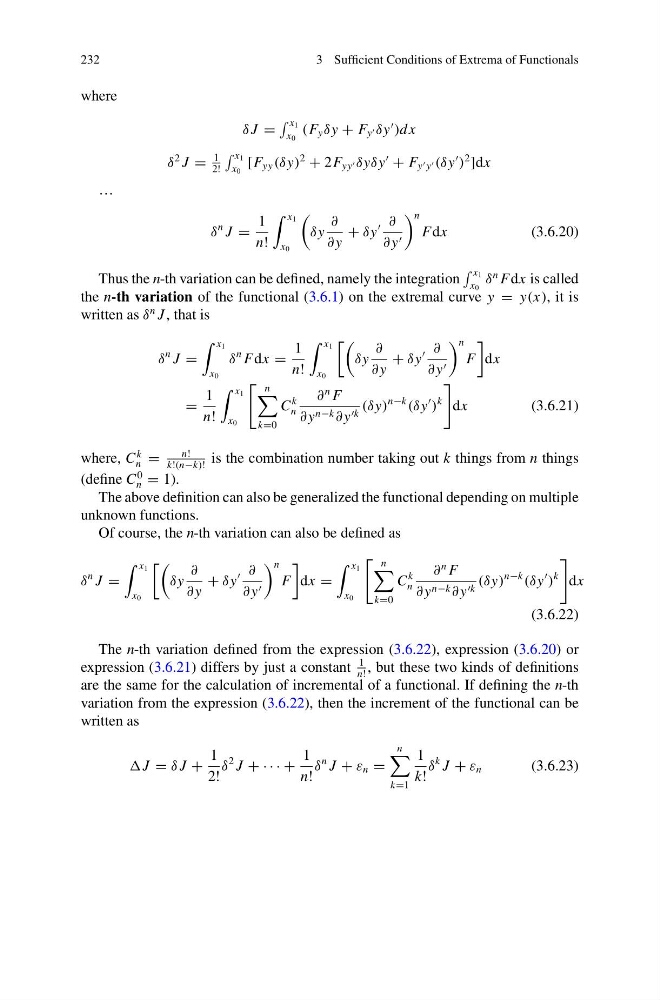
Thus the n-th variation can be defined, namely the integration
x 1
x 0
δ
n Fdx is called
the n-th variation of the functional (3.6.1) on the extremal curve y = y(x), it is
written as δ
n J , that is
δ
n J =
x 1
x 0
δ
n Fdx =
1
n!
x 1
x 0
δy
∂
∂ y
+ δy
∂
∂ y
n
F
dx
=
1
n!
x 1
x 0
n
k=0
C
k
n
∂
n F
∂ y n−k ∂ y k (δy)
n−k
(δy
)
k
dx
(3.6.21)
where, C
k
n =
n!
k!(n−k)!
is the combination number taking out k things from n things
(define C
0
n = 1).
The above definition can also be generalized the functional depending on multiple
unknown functions.
Of course, the n-th variation can also be defined as
δ
n J =
x 1
x 0
δy
∂
∂ y
+ δy
∂
∂ y
n
F
dx =
x 1
x 0
n
k=0
C
k
n
∂
n F
∂ y n−k ∂ y k (δy)
n−k
(δy
)
k
dx
(3.6.22)
The n-th variation defined from the expression (3.6.22), expression (3.6.20) or
expression (3.6.21) differs by just a constant
1
n!
, but these two kinds of definitions
are the same for the calculation of incremental of a functional. If defining the n-th
variation from the expression (3.6.22), then the increment of the functional can be
written as
J = δ J +
1
2!
δ
2 J + · · · +
1
n!
δ
n J + ε n =
n
k=1
1
k!
δ
k J + ε n
(3.6.23)
3 Sufficient Conditions of Extrema of Functionals
where
δ J =
x 1
x 0
(F y δy + F y δy
)dx
δ
2 J =
1
2!
x 1
x 0
[F yy (δy)
2
+ 2F yy δyδy
+ F y y (δy
)
2
]dx
…
δ
n J =
1
n!
x 1
x 0
δy
∂
∂ y
+ δy
∂
∂ y
n
Fdx
(3.6.20)
Thus the n-th variation can be defined, namely the integration
x 1
x 0
δ
n Fdx is called
the n-th variation of the functional (3.6.1) on the extremal curve y = y(x), it is
written as δ
n J , that is
δ
n J =
x 1
x 0
δ
n Fdx =
1
n!
x 1
x 0
δy
∂
∂ y
+ δy
∂
∂ y
n
F
dx
=
1
n!
x 1
x 0
n
k=0
C
k
n
∂
n F
∂ y n−k ∂ y k (δy)
n−k
(δy
)
k
dx
(3.6.21)
where, C
k
n =
n!
k!(n−k)!
is the combination number taking out k things from n things
(define C
0
n = 1).
The above definition can also be generalized the functional depending on multiple
unknown functions.
Of course, the n-th variation can also be defined as
δ
n J =
x 1
x 0
δy
∂
∂ y
+ δy
∂
∂ y
n
F
dx =
x 1
x 0
n
k=0
C
k
n
∂
n F
∂ y n−k ∂ y k (δy)
n−k
(δy
)
k
dx
(3.6.22)
The n-th variation defined from the expression (3.6.22), expression (3.6.20) or
expression (3.6.21) differs by just a constant
1
n!
, but these two kinds of definitions
are the same for the calculation of incremental of a functional. If defining the n-th
variation from the expression (3.6.22), then the increment of the functional can be
written as
J = δ J +
1
2!
δ
2 J + · · · +
1
n!
δ
n J + ε n =
n
k=1
1
k!
δ
k J + ε n
(3.6.23)