

230
3 Sufficient Conditions of Extrema of Functionals
Thus
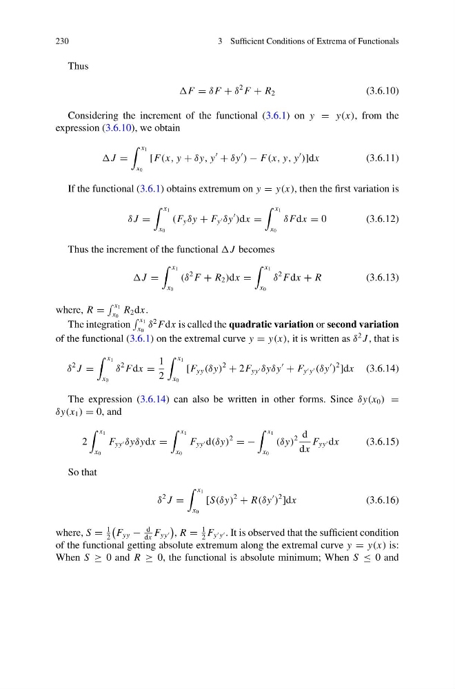
F = δ F + δ
2 F + R 2
(3.6.10)
Considering the increment of the functional (3.6.1) on y = y(x), from the
expression (3.6.10), we obtain
J =
x 1
x 0
[F(x, y + δy, y
+ δy
) − F(x, y, y
)]dx
(3.6.11)
If the functional (3.6.1) obtains extremum on y = y(x), then the first variation is
δ J =
x 1
x 0
(F y δy + F y δy
)dx =
x 1
x 0
δ Fdx = 0
(3.6.12)
Thus the increment of the functional J becomes
J =
x 1
x 0
(δ
2 F + R 2 )dx =
x 1
x 0
δ
2 Fdx + R
(3.6.13)
where, R =
x 1
x 0
R 2 dx.
The integration
x 1
x 0
δ
2 Fdx is called the quadratic variation or second variation
of the functional (3.6.1) on the extremal curve y = y(x), it is written as δ
2 J , that is
δ
2 J =
x 1
x 0
δ
2 Fdx =
1
2
x 1
x 0
[F yy (δy)
2
+ 2F yy δyδy
+ F y y (δy
)
2
]dx (3.6.14)
The expression (3.6.14) can also be written in other forms. Since δy(x 0 ) =
δy(x 1 ) = 0, and
2
x 1
x 0
F yy δyδydx =
x 1
x 0
F yy d(δy)
2
= −
x 1
x 0
(δy)
2 d
dx
F yy dx
(3.6.15)
So that
δ
2 J =
x 1
x 0
[S(δy)
2
+ R(δy
)
2
]dx
(3.6.16)
where, S =
1
2
F yy −
d
dx
F yy
, R =
1
2
F y y . It is observed that the sufficient condition
of the functional getting absolute extremum along the extremal curve y = y(x) is:
When S ≥ 0 and R ≥ 0, the functional is absolute minimum; When S ≤ 0 and
3 Sufficient Conditions of Extrema of Functionals
Thus
F = δ F + δ
2 F + R 2
(3.6.10)
Considering the increment of the functional (3.6.1) on y = y(x), from the
expression (3.6.10), we obtain
J =
x 1
x 0
[F(x, y + δy, y
+ δy
) − F(x, y, y
)]dx
(3.6.11)
If the functional (3.6.1) obtains extremum on y = y(x), then the first variation is
δ J =
x 1
x 0
(F y δy + F y δy
)dx =
x 1
x 0
δ Fdx = 0
(3.6.12)
Thus the increment of the functional J becomes
J =
x 1
x 0
(δ
2 F + R 2 )dx =
x 1
x 0
δ
2 Fdx + R
(3.6.13)
where, R =
x 1
x 0
R 2 dx.
The integration
x 1
x 0
δ
2 Fdx is called the quadratic variation or second variation
of the functional (3.6.1) on the extremal curve y = y(x), it is written as δ
2 J , that is
δ
2 J =
x 1
x 0
δ
2 Fdx =
1
2
x 1
x 0
[F yy (δy)
2
+ 2F yy δyδy
+ F y y (δy
)
2
]dx (3.6.14)
The expression (3.6.14) can also be written in other forms. Since δy(x 0 ) =
δy(x 1 ) = 0, and
2
x 1
x 0
F yy δyδydx =
x 1
x 0
F yy d(δy)
2
= −
x 1
x 0
(δy)
2 d
dx
F yy dx
(3.6.15)
So that
δ
2 J =
x 1
x 0
[S(δy)
2
+ R(δy
)
2
]dx
(3.6.16)
where, S =
1
2
F yy −
d
dx
F yy
, R =
1
2
F y y . It is observed that the sufficient condition
of the functional getting absolute extremum along the extremal curve y = y(x) is:
When S ≥ 0 and R ≥ 0, the functional is absolute minimum; When S ≤ 0 and