

224
3 Sufficient Conditions of Extrema of Functionals
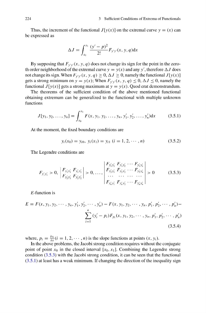
Thus, the increment of the functional J [y(x)] on the extremal curve y = (x) can
be expressed as
J =
x 1
x 0
(y
− p)
2
2!
F y y (x, y, q)dx
By supposing that F y y (x, y, q) does not change its sign for the point in the zeroth order neighborhood of the extremal curve y = y(x) and any y
, therefore J does
not change its sign. When F y y (x, y, q) ≥ 0, J ≥ 0, namely the functional J [y(x)]
gets a strong minimum on y = y(x); When F y y (x, y, q) ≤ 0, J ≤ 0, namely the
functional J [y(x)] gets a strong maximum at y = y(x). Quod erat demonstrandum.
The theorems of the sufficient condition of the above mentioned functional
obtaining extremum can be generalized to the functional with multiple unknown
functions
J [y 1 , y 2 , . . . , y n ] =
x 1
x 0
F(x, y 1 , y 2 , . . . , y n , y
1 , y
2 , . . . , y
n )dx
(3.5.1)
At the moment, the fixed boundary conditions are
y i (x 0 ) = y i0 , y i (x 1 ) = y i1 (i = 1, 2, · · · , n)
(3.5.2)
The Legendre conditions are
F y
1 y
1
> 0,
F y
1 y
1
F y
1 y
2
F y
2 y
1
F y
2 y
2
> 0, . . . ,
F y
1 y
1
F y
1 y
2
· · · F y
1 y
n
F y
2 y
1
F y
2 y
2
· · · F y
2 y
n
· · · · · · · · · · · ·
F y
n y
1
F y
n y
2
· · · F y
n y
n
> 0
(3.5.3)
E-function is
E = F(x, y 1 , y 2 , · · · , y n , y
1 , y
2 , · · · , y
n ) − F(x, y 1 , y 2 , · · · , y n , p
1 , p
2 , · · · , p
n )−
n
i=1
(y
i − p i )F p i (x, y 1 , y 2 , · · · , y n , p
1 , p
2 , · · · , p
n )
(3.5.4)
where, p i =
∂ y i
∂ x
(i = 1, 2, · · · , n) is the slope functions at points (x, y i ).
In the above problems, the Jacobi strong condition requires without the conjugate
point of point x 0 in the closed interval [x 0 , x 1 ]. Combining the Legendre strong
condition (3.5.3) with the Jacobi strong condition, it can be seen that the functional
(3.5.1) at least has a weak minimum. If changing the direction of the inequality sign
3 Sufficient Conditions of Extrema of Functionals
Thus, the increment of the functional J [y(x)] on the extremal curve y = (x) can
be expressed as
J =
x 1
x 0
(y
− p)
2
2!
F y y (x, y, q)dx
By supposing that F y y (x, y, q) does not change its sign for the point in the zeroth order neighborhood of the extremal curve y = y(x) and any y
, therefore J does
not change its sign. When F y y (x, y, q) ≥ 0, J ≥ 0, namely the functional J [y(x)]
gets a strong minimum on y = y(x); When F y y (x, y, q) ≤ 0, J ≤ 0, namely the
functional J [y(x)] gets a strong maximum at y = y(x). Quod erat demonstrandum.
The theorems of the sufficient condition of the above mentioned functional
obtaining extremum can be generalized to the functional with multiple unknown
functions
J [y 1 , y 2 , . . . , y n ] =
x 1
x 0
F(x, y 1 , y 2 , . . . , y n , y
1 , y
2 , . . . , y
n )dx
(3.5.1)
At the moment, the fixed boundary conditions are
y i (x 0 ) = y i0 , y i (x 1 ) = y i1 (i = 1, 2, · · · , n)
(3.5.2)
The Legendre conditions are
F y
1 y
1
> 0,
F y
1 y
1
F y
1 y
2
F y
2 y
1
F y
2 y
2
> 0, . . . ,
F y
1 y
1
F y
1 y
2
· · · F y
1 y
n
F y
2 y
1
F y
2 y
2
· · · F y
2 y
n
· · · · · · · · · · · ·
F y
n y
1
F y
n y
2
· · · F y
n y
n
> 0
(3.5.3)
E-function is
E = F(x, y 1 , y 2 , · · · , y n , y
1 , y
2 , · · · , y
n ) − F(x, y 1 , y 2 , · · · , y n , p
1 , p
2 , · · · , p
n )−
n
i=1
(y
i − p i )F p i (x, y 1 , y 2 , · · · , y n , p
1 , p
2 , · · · , p
n )
(3.5.4)
where, p i =
∂ y i
∂ x
(i = 1, 2, · · · , n) is the slope functions at points (x, y i ).
In the above problems, the Jacobi strong condition requires without the conjugate
point of point x 0 in the closed interval [x 0 , x 1 ]. Combining the Legendre strong
condition (3.5.3) with the Jacobi strong condition, it can be seen that the functional
(3.5.1) at least has a weak minimum. If changing the direction of the inequality sign