

204
3 Sufficient Conditions of Extrema of Functionals
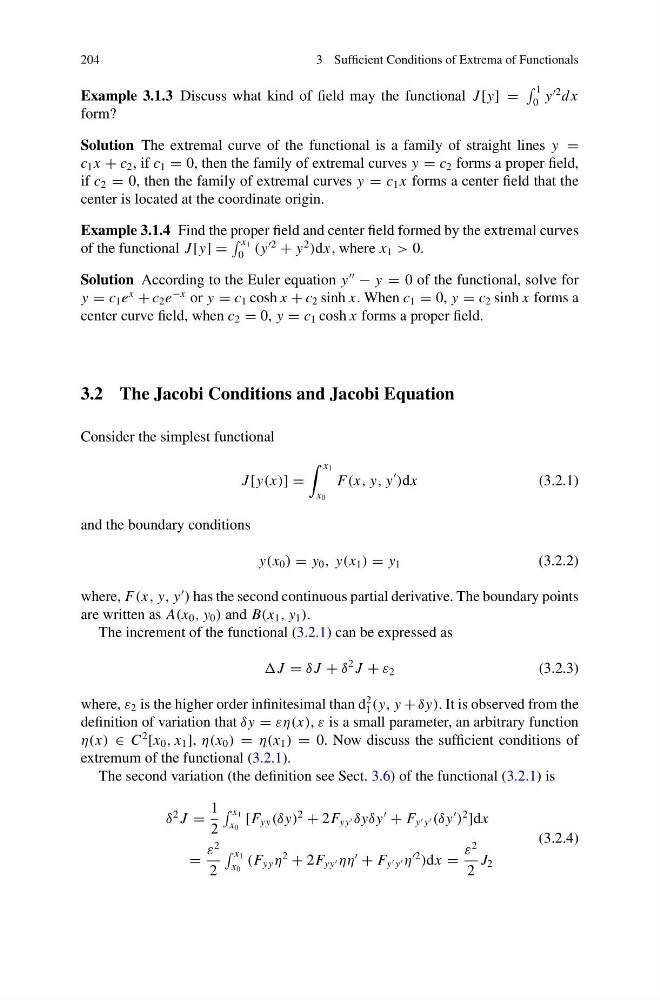
Example 3.1.3 Discuss what kind of field may the functional J [y] =
1
0 y
2 dx
form?
Solution The extremal curve of the functional is a family of straight lines y =
c 1 x + c 2 , if c 1 = 0, then the family of extremal curves y = c 2 forms a proper field,
if c 2 = 0, then the family of extremal curves y = c 1 x forms a center field that the
center is located at the coordinate origin.
Example 3.1.4 Find the proper field and center field formed by the extremal curves
of the functional J [y] =
x 1
0 (y
2
+ y
2
)dx, where x 1 > 0.
Solution According to the Euler equation y
− y = 0 of the functional, solve for
y = c 1 e
x
+ c 2 e
−x or y = c 1 cosh x + c 2 sinh x. When c 1 = 0, y = c 2 sinh x forms a
center curve field, when c 2 = 0, y = c 1 cosh x forms a proper field.
3.2 The Jacobi Conditions and Jacobi Equation
Consider the simplest functional
J [y(x)] =
x 1
x 0
F(x, y, y
)dx
(3.2.1)
and the boundary conditions
y(x 0 ) = y 0 , y(x 1 ) = y 1
(3.2.2)
where, F(x, y, y
) has the second continuous partial derivative. The boundary points
are written as A(x 0 , y 0 ) and B(x 1 , y 1 ).
The increment of the functional (3.2.1) can be expressed as
J = δ J + δ
2 J + ε 2
(3.2.3)
where, ε 2 is the higher order infinitesimal than d
2
1 (y, y + δy). It is observed from the
definition of variation that δy = εη(x), ε is a small parameter, an arbitrary function
η(x) ∈ C
2
[x 0 , x 1 ], η(x 0 ) = η(x 1 ) = 0. Now discuss the sufficient conditions of
extremum of the functional (3.2.1).
The second variation (the definition see Sect. 3.6) of the functional (3.2.1) is
δ
2 J =
1
2
x 1
x 0
[F yy (δy)
2
+ 2F yy δyδy
+ F y y (δy
)
2
]dx
=
ε
2
2
x 1
x 0
(F yy η
2
+ 2F yy ηη
+ F y y η
2
)dx =
ε
2
2
J 2
(3.2.4)
3 Sufficient Conditions of Extrema of Functionals
Example 3.1.3 Discuss what kind of field may the functional J [y] =
1
0 y
2 dx
form?
Solution The extremal curve of the functional is a family of straight lines y =
c 1 x + c 2 , if c 1 = 0, then the family of extremal curves y = c 2 forms a proper field,
if c 2 = 0, then the family of extremal curves y = c 1 x forms a center field that the
center is located at the coordinate origin.
Example 3.1.4 Find the proper field and center field formed by the extremal curves
of the functional J [y] =
x 1
0 (y
2
+ y
2
)dx, where x 1 > 0.
Solution According to the Euler equation y
− y = 0 of the functional, solve for
y = c 1 e
x
+ c 2 e
−x or y = c 1 cosh x + c 2 sinh x. When c 1 = 0, y = c 2 sinh x forms a
center curve field, when c 2 = 0, y = c 1 cosh x forms a proper field.
3.2 The Jacobi Conditions and Jacobi Equation
Consider the simplest functional
J [y(x)] =
x 1
x 0
F(x, y, y
)dx
(3.2.1)
and the boundary conditions
y(x 0 ) = y 0 , y(x 1 ) = y 1
(3.2.2)
where, F(x, y, y
) has the second continuous partial derivative. The boundary points
are written as A(x 0 , y 0 ) and B(x 1 , y 1 ).
The increment of the functional (3.2.1) can be expressed as
J = δ J + δ
2 J + ε 2
(3.2.3)
where, ε 2 is the higher order infinitesimal than d
2
1 (y, y + δy). It is observed from the
definition of variation that δy = εη(x), ε is a small parameter, an arbitrary function
η(x) ∈ C
2
[x 0 , x 1 ], η(x 0 ) = η(x 1 ) = 0. Now discuss the sufficient conditions of
extremum of the functional (3.2.1).
The second variation (the definition see Sect. 3.6) of the functional (3.2.1) is
δ
2 J =
1
2
x 1
x 0
[F yy (δy)
2
+ 2F yy δyδy
+ F y y (δy
)
2
]dx
=
ε
2
2
x 1
x 0
(F yy η
2
+ 2F yy ηη
+ F y y η
2
)dx =
ε
2
2
J 2
(3.2.4)