

180
2 Variational Problems with Fixed Boundaries
J [y] =
ξ 1
ξ 0
G
ξ, y,
dy
dξ
dx
dξ
dξ
(2.10.9)
Moreover let
H
ξ, y,
dy
dξ
= G
ξ, y,
dy
dξ
dx
dξ
(2.10.10)
then there is
J [y] =
ξ 1
ξ 0
H
ξ, y,
dy
dξ
dξ
(2.10.11)
The Euler equation is
H y −
d
dξ
H dy
dξ
= 0
(2.10.12)
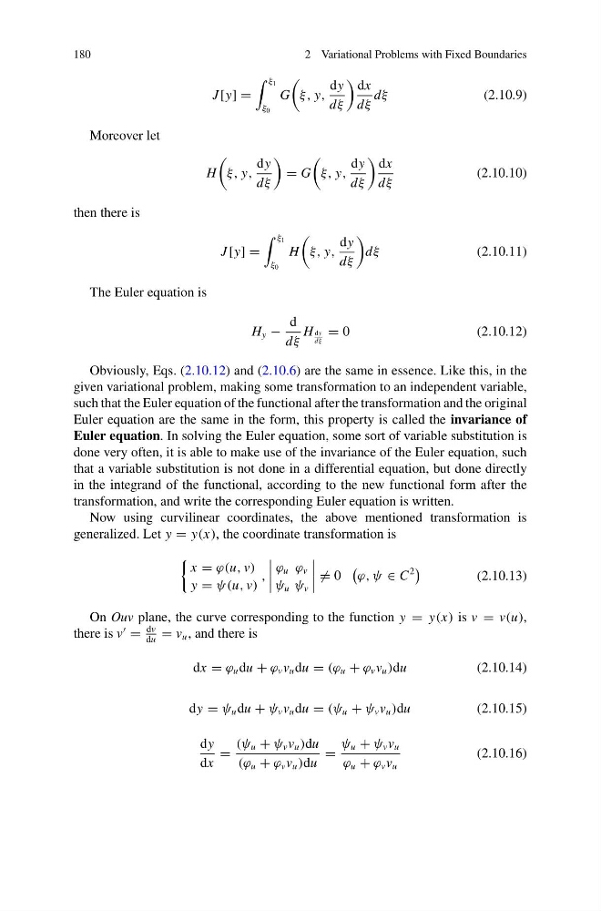
Obviously, Eqs. (2.10.12) and (2.10.6) are the same in essence. Like this, in the
given variational problem, making some transformation to an independent variable,
such that the Euler equation of the functional after the transformation and the original
Euler equation are the same in the form, this property is called the invariance of
Euler equation. In solving the Euler equation, some sort of variable substitution is
done very often, it is able to make use of the invariance of the Euler equation, such
that a variable substitution is not done in a differential equation, but done directly
in the integrand of the functional, according to the new functional form after the
transformation, and write the corresponding Euler equation is written.
Now using curvilinear coordinates, the above mentioned transformation is
generalized. Let y = y(x), the coordinate transformation is
x = ϕ(u, v)
y = ψ(u, v)
,
ϕ u ϕ v
ψ u ψ v
= 0
ϕ, ψ ∈ C
2
(2.10.13)
On Ouv plane, the curve corresponding to the function y = y(x) is v = v(u),
there is v
=
dv
du
= v u , and there is
dx = ϕ u du + ϕ v v u du = (ϕ u + ϕ v v u )du
(2.10.14)
dy = ψ u du + ψ v v u du = (ψ u + ψ v v u )du
(2.10.15)
dy
dx
=
(ψ u + ψ v v u )du
(ϕ u + ϕ v v u )du
=
ψ u + ψ v v u
ϕ u + ϕ v v u
(2.10.16)
2 Variational Problems with Fixed Boundaries
J [y] =
ξ 1
ξ 0
G
ξ, y,
dy
dξ
dx
dξ
dξ
(2.10.9)
Moreover let
H
ξ, y,
dy
dξ
= G
ξ, y,
dy
dξ
dx
dξ
(2.10.10)
then there is
J [y] =
ξ 1
ξ 0
H
ξ, y,
dy
dξ
dξ
(2.10.11)
The Euler equation is
H y −
d
dξ
H dy
dξ
= 0
(2.10.12)
Obviously, Eqs. (2.10.12) and (2.10.6) are the same in essence. Like this, in the
given variational problem, making some transformation to an independent variable,
such that the Euler equation of the functional after the transformation and the original
Euler equation are the same in the form, this property is called the invariance of
Euler equation. In solving the Euler equation, some sort of variable substitution is
done very often, it is able to make use of the invariance of the Euler equation, such
that a variable substitution is not done in a differential equation, but done directly
in the integrand of the functional, according to the new functional form after the
transformation, and write the corresponding Euler equation is written.
Now using curvilinear coordinates, the above mentioned transformation is
generalized. Let y = y(x), the coordinate transformation is
x = ϕ(u, v)
y = ψ(u, v)
,
ϕ u ϕ v
ψ u ψ v
= 0
ϕ, ψ ∈ C
2
(2.10.13)
On Ouv plane, the curve corresponding to the function y = y(x) is v = v(u),
there is v
=
dv
du
= v u , and there is
dx = ϕ u du + ϕ v v u du = (ϕ u + ϕ v v u )du
(2.10.14)
dy = ψ u du + ψ v v u du = (ψ u + ψ v v u )du
(2.10.15)
dy
dx
=
(ψ u + ψ v v u )du
(ϕ u + ϕ v v u )du
=
ψ u + ψ v v u
ϕ u + ϕ v v u
(2.10.16)