

2.9 Variational Problems of Complete Function
175
δ J =
S
s=1
B s +
Ω
F u +
S
s=1
(−1)
i s D
i s F D is u
δudx 1 dx 2 · · · dx m = 0 (2.9.9)
where, from the necessary condition δ J = 0 of extremum of a functional, there
should be
S
s=1
B s = 0 and the integral term is equal to zero, and according to the fundamental lemma of variational methods, δu is arbitrary, the parts in square brackets of
the integral term can only be equal to zero, thus Eqs. (2.9.5)–(2.9.8) can be obtained.
Quod erat demonstrandum.
Equations (2.9.5)–(2.9.8) have two laws, one law is that there are two same operators in sum term, This shows that after taking partial derivative of F with respect to
a derivative term with some independent variables, to take taking partial derivative
with respect to these independent variables again, namely the two groups of independent variables of partial derivative with respect to the independent variables are the
same. Another law is about the symbol of each term in the summation term, making
integration by parts once, the integrand is changed the sign once, thus odd integrals
are negative sign, even integrals are positive sign, this law can be expressed by i s ,
when i s is an even, the integrand is positive sign, when i s is an odd, the integrand is
negative sign. To master the two laws will bring great convenience for the application
of the above mentioned formulas.
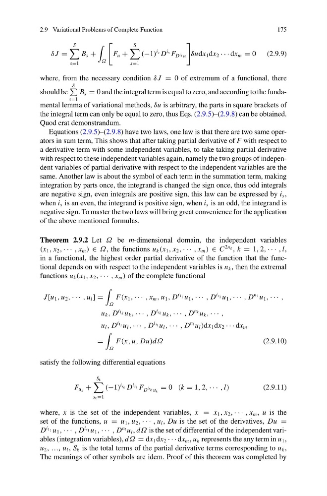
Theorem 2.9.2 Let Ω be m-dimensional domain, the independent variables
(x 1 , x 2 , · · · , x m ) ∈ Ω, the functions u k (x 1 , x 2 , · · · , x m ) ∈ C
2n k , k = 1, 2, · · · , l,
in a functional, the highest order partial derivative of the function that the functional depends on with respect to the independent variables is n k , then the extremal
functions u k (x 1 , x 2 , · · · , x m ) of the complete functional
J [u 1 , u 2 , · · · , u l ] =
Ω
F(x 1 , · · · , x m , u 1 , D
i 1 1 u 1 , · · · , D
i s 1 u 1 , · · · , D
n 1 u 1 , · · · ,
u k , D
i 1 k u k , · · · , D
i s k u k , · · · , D
n k u k , · · · ,
u l , D
i 1 l u l , · · · , D
i s l u l , · · · , D
n l u l )dx 1 dx 2 · · · dx m
=
Ω
F(x, u, Du)dΩ
(2.9.10)
satisfy the following differential equations
F u k +
S k
s k =1
(−1)
i s k D
i s k F D
is k u k
= 0 (k = 1, 2, · · · , l)
(2.9.11)
where, x is the set of the independent variables, x = x 1 , x 2 , · · · , x m , u is the
set of the functions, u = u 1 , u 2 , · · · , u l , Du is the set of the derivatives, Du =
D
i 1 1 u 1 , · · · , D
i s 1 u 1 , · · · , D
n l u l , dΩ is the set of differential of the independent variables (integration variables), dΩ = dx 1 dx 2 · · · dx m , u k represents the any term in u 1 ,
u 2 , …, u l , S k is the total terms of the partial derivative terms corresponding to u k ,
The meanings of other symbols are idem. Proof of this theorem was completed by
175
δ J =
S
s=1
B s +
Ω
F u +
S
s=1
(−1)
i s D
i s F D is u
δudx 1 dx 2 · · · dx m = 0 (2.9.9)
where, from the necessary condition δ J = 0 of extremum of a functional, there
should be
S
s=1
B s = 0 and the integral term is equal to zero, and according to the fundamental lemma of variational methods, δu is arbitrary, the parts in square brackets of
the integral term can only be equal to zero, thus Eqs. (2.9.5)–(2.9.8) can be obtained.
Quod erat demonstrandum.
Equations (2.9.5)–(2.9.8) have two laws, one law is that there are two same operators in sum term, This shows that after taking partial derivative of F with respect to
a derivative term with some independent variables, to take taking partial derivative
with respect to these independent variables again, namely the two groups of independent variables of partial derivative with respect to the independent variables are the
same. Another law is about the symbol of each term in the summation term, making
integration by parts once, the integrand is changed the sign once, thus odd integrals
are negative sign, even integrals are positive sign, this law can be expressed by i s ,
when i s is an even, the integrand is positive sign, when i s is an odd, the integrand is
negative sign. To master the two laws will bring great convenience for the application
of the above mentioned formulas.
Theorem 2.9.2 Let Ω be m-dimensional domain, the independent variables
(x 1 , x 2 , · · · , x m ) ∈ Ω, the functions u k (x 1 , x 2 , · · · , x m ) ∈ C
2n k , k = 1, 2, · · · , l,
in a functional, the highest order partial derivative of the function that the functional depends on with respect to the independent variables is n k , then the extremal
functions u k (x 1 , x 2 , · · · , x m ) of the complete functional
J [u 1 , u 2 , · · · , u l ] =
Ω
F(x 1 , · · · , x m , u 1 , D
i 1 1 u 1 , · · · , D
i s 1 u 1 , · · · , D
n 1 u 1 , · · · ,
u k , D
i 1 k u k , · · · , D
i s k u k , · · · , D
n k u k , · · · ,
u l , D
i 1 l u l , · · · , D
i s l u l , · · · , D
n l u l )dx 1 dx 2 · · · dx m
=
Ω
F(x, u, Du)dΩ
(2.9.10)
satisfy the following differential equations
F u k +
S k
s k =1
(−1)
i s k D
i s k F D
is k u k
= 0 (k = 1, 2, · · · , l)
(2.9.11)
where, x is the set of the independent variables, x = x 1 , x 2 , · · · , x m , u is the
set of the functions, u = u 1 , u 2 , · · · , u l , Du is the set of the derivatives, Du =
D
i 1 1 u 1 , · · · , D
i s 1 u 1 , · · · , D
n l u l , dΩ is the set of differential of the independent variables (integration variables), dΩ = dx 1 dx 2 · · · dx m , u k represents the any term in u 1 ,
u 2 , …, u l , S k is the total terms of the partial derivative terms corresponding to u k ,
The meanings of other symbols are idem. Proof of this theorem was completed by