

92
2 Variational Problems with Fixed Boundaries
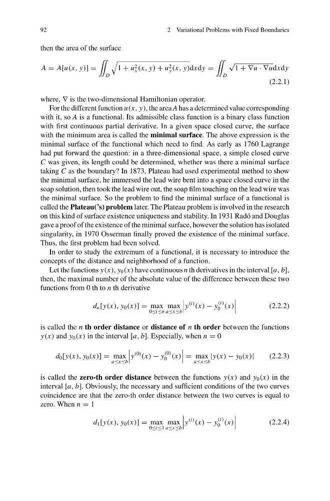
then the area of the surface
A = A[u(x, y)] =
¨
D
1 + u 2
x (x, y) + u 2
y (x, y)dxdy =
¨
D
√
1 + ∇u · ∇udxdy
(2.2.1)
where, ∇ is the two-dimensional Hamiltonian operator.
For the different function u(x, y), the area A has a determined value corresponding
with it, so A is a functional. Its admissible class function is a binary class function
with first continuous partial derivative. In a given space closed curve, the surface
with the minimum area is called the minimal surface. The above expression is the
minimal surface of the functional which need to find. As early as 1760 Lagrange
had put forward the question: in a three-dimensional space, a simple closed curve
C was given, its length could be determined, whether was there a minimal surface
taking C as the boundary? In 1873, Plateau had used experimental method to show
the minimal surface, he immersed the lead wire bent into a space closed curve in the
soap solution, then took the lead wire out, the soap film touching on the lead wire was
the minimal surface. So the problem to find the minimal surface of a functional is
called the Plateau(’s) problem later. The Plateau problem is involved in the research
on this kind of surface existence uniqueness and stability. In 1931 Radó and Douglas
gave a proof of the existence of the minimal surface, however the solution has isolated
singularity, in 1970 Osserman finally proved the existence of the minimal surface.
Thus, the first problem had been solved.
In order to study the extremum of a functional, it is necessary to introduce the
concepts of the distance and neighborhood of a function.
Let the functions y(x), y 0 (x) have continuous n th derivatives in the interval [a, b],
then, the maximal number of the absolute value of the difference between these two
functions from 0 th to n th derivative
d n [y(x), y 0 (x)] = max
0≤i≤n
max
a≤x≤b
y
(i)
(x) − y
(i)
0 (x)
(2.2.2)
is called the n th order distance or distance of n th order between the functions
y(x) and y 0 (x) in the interval [a, b]. Especially, when n = 0
d 0 [y(x), y 0 (x)] = max
a≤x≤b
y
(0)
(x) − y
(0)
0 (x)
= max
a≤x≤b
|y(x) − y 0 (x)|
(2.2.3)
is called the zero-th order distance between the functions y(x) and y 0 (x) in the
interval [a, b]. Obviously, the necessary and sufficient conditions of the two curves
coincidence are that the zero-th order distance between the two curves is equal to
zero. When n = 1
d 1 [y(x), y 0 (x)] = max
0≤i≤1
max
a≤x≤b
y
(i)
(x) − y
(i)
0 (x)
(2.2.4)
2 Variational Problems with Fixed Boundaries
then the area of the surface
A = A[u(x, y)] =
¨
D
1 + u 2
x (x, y) + u 2
y (x, y)dxdy =
¨
D
√
1 + ∇u · ∇udxdy
(2.2.1)
where, ∇ is the two-dimensional Hamiltonian operator.
For the different function u(x, y), the area A has a determined value corresponding
with it, so A is a functional. Its admissible class function is a binary class function
with first continuous partial derivative. In a given space closed curve, the surface
with the minimum area is called the minimal surface. The above expression is the
minimal surface of the functional which need to find. As early as 1760 Lagrange
had put forward the question: in a three-dimensional space, a simple closed curve
C was given, its length could be determined, whether was there a minimal surface
taking C as the boundary? In 1873, Plateau had used experimental method to show
the minimal surface, he immersed the lead wire bent into a space closed curve in the
soap solution, then took the lead wire out, the soap film touching on the lead wire was
the minimal surface. So the problem to find the minimal surface of a functional is
called the Plateau(’s) problem later. The Plateau problem is involved in the research
on this kind of surface existence uniqueness and stability. In 1931 Radó and Douglas
gave a proof of the existence of the minimal surface, however the solution has isolated
singularity, in 1970 Osserman finally proved the existence of the minimal surface.
Thus, the first problem had been solved.
In order to study the extremum of a functional, it is necessary to introduce the
concepts of the distance and neighborhood of a function.
Let the functions y(x), y 0 (x) have continuous n th derivatives in the interval [a, b],
then, the maximal number of the absolute value of the difference between these two
functions from 0 th to n th derivative
d n [y(x), y 0 (x)] = max
0≤i≤n
max
a≤x≤b
y
(i)
(x) − y
(i)
0 (x)
(2.2.2)
is called the n th order distance or distance of n th order between the functions
y(x) and y 0 (x) in the interval [a, b]. Especially, when n = 0
d 0 [y(x), y 0 (x)] = max
a≤x≤b
y
(0)
(x) − y
(0)
0 (x)
= max
a≤x≤b
|y(x) − y 0 (x)|
(2.2.3)
is called the zero-th order distance between the functions y(x) and y 0 (x) in the
interval [a, b]. Obviously, the necessary and sufficient conditions of the two curves
coincidence are that the zero-th order distance between the two curves is equal to
zero. When n = 1
d 1 [y(x), y 0 (x)] = max
0≤i≤1
max
a≤x≤b
y
(i)
(x) − y
(i)
0 (x)
(2.2.4)