

2.1 Examples of the Classical Variational Problems
87
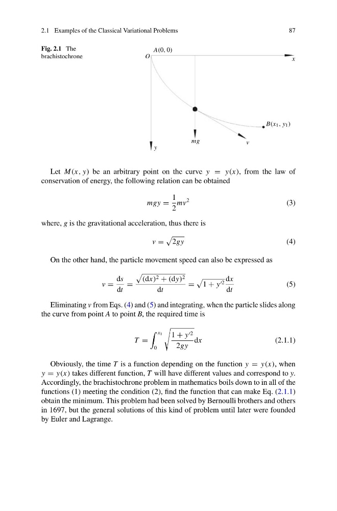
Fig. 2.1 The
brachistochrone
O
x
y
A(0, 0)
B(x 1 , y 1 )
mg
v
Let M(x, y) be an arbitrary point on the curve y = y(x), from the law of
conservation of energy, the following relation can be obtained
mgy =
1
2
mv
2
(3)
where, g is the gravitational acceleration, thus there is
v =
2gy
(4)
On the other hand, the particle movement speed can also be expressed as
v =
ds
dt
=
(dx) 2 + (dy) 2
dt
=
1 + y dx
dt
(5)
Eliminating v from Eqs. (4) and (5) and integrating, when the particle slides along
the curve from point A to point B, the required time is
T =
x 1
0
1 + y
2gy
dx
(2.1.1)
Obviously, the time T is a function depending on the function y = y(x), when
y = y(x) takes different function, T will have different values and correspond to y.
Accordingly, the brachistochrone problem in mathematics boils down to in all of the
functions (1) meeting the condition (2), find the function that can make Eq. (2.1.1)
obtain the minimum. This problem had been solved by Bernoulli brothers and others
in 1697, but the general solutions of this kind of problem until later were founded
by Euler and Lagrange.
87
Fig. 2.1 The
brachistochrone
O
x
y
A(0, 0)
B(x 1 , y 1 )
mg
v
Let M(x, y) be an arbitrary point on the curve y = y(x), from the law of
conservation of energy, the following relation can be obtained
mgy =
1
2
mv
2
(3)
where, g is the gravitational acceleration, thus there is
v =
2gy
(4)
On the other hand, the particle movement speed can also be expressed as
v =
ds
dt
=
(dx) 2 + (dy) 2
dt
=
1 + y dx
dt
(5)
Eliminating v from Eqs. (4) and (5) and integrating, when the particle slides along
the curve from point A to point B, the required time is
T =
x 1
0
1 + y
2gy
dx
(2.1.1)
Obviously, the time T is a function depending on the function y = y(x), when
y = y(x) takes different function, T will have different values and correspond to y.
Accordingly, the brachistochrone problem in mathematics boils down to in all of the
functions (1) meeting the condition (2), find the function that can make Eq. (2.1.1)
obtain the minimum. This problem had been solved by Bernoulli brothers and others
in 1697, but the general solutions of this kind of problem until later were founded
by Euler and Lagrange.