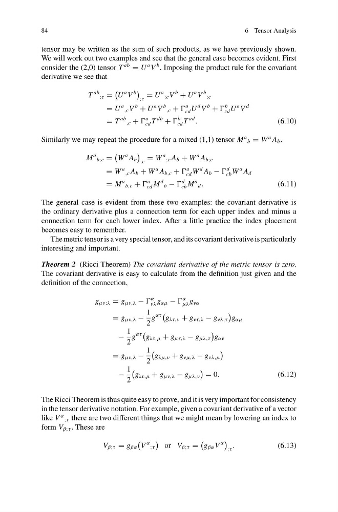
84
6 Tensor Analysis
tensor may be written as the sum of such products, as we have previously shown.
We will work out two examples and see that the general case becomes evident. First
consider the (2,0) tensor T
ab
= U
a V
b . Imposing the product rule for the covariant
derivative we see that
T
ab ;c =
U
a V
b
;c
= U
a ;c V
b
+ U
a V
b ;c
= U
a ,c V
b
+ U
a V
b ,c +
a
cd U
d V
b
+
b
cd U
a V
d
= T
ab ,c +
a
cd T
db
+
b
cd T
ad
.
(6.10)
Similarly we may repeat the procedure for a mixed (1,1) tensor M
a
b = W
a A b .
M
a
b;c =
W
a A b
;c
= W
a ;c A b + W
a A b;c
= W
a ,c A b + W
a A b,c +
a
cd W
d A b −
d
cb W
a A d
= M
a
b,c +
a
cd M
d
b −
d
cb M
a
d .
(6.11)
The general case is evident from these two examples: the covariant derivative is
the ordinary derivative plus a connection term for each upper index and minus a
connection term for each lower index. After a little practice the index placement
becomes easy to remember.
The metric tensor is a very special tensor, and its covariant derivative is particularly
interesting and important.
Theorem 2 (Ricci Theorem) The covariant derivative of the metric tensor is zero.
The covariant derivative is easy to calculate from the definition just given and the
definition of the connection,
g μν;λ = g μν,λ −
α
νλ g αμ −
α
μλ g να
= g μν,λ −
1
2
g
ατ
g λτ,ν + g ντ,λ − g νλ,τ
g αμ
−
1
2
g
ατ
g λτ,μ + g μτ,λ − g μλ,τ
g αν
= g μν,λ −
1
2
g λμ,ν + g νμ,λ − g νλ,μ
−
1
2
g λν,μ + g μν,λ − g μλ,ν
= 0.
(6.12)
The Ricci Theorem is thus quite easy to prove, and it is very important for consistency
in the tensor derivative notation. For example, given a covariant derivative of a vector
like V
α ;τ there are two different things that we might mean by lowering an index to
form V β;τ . These are
V β;τ = g βα
V
α ;τ
or V β;τ =
g βα V
α
;τ
.
(6.13)