

76
5 Affine Connections and Geodesics
Appendix 2: The Extremum Problem
and the Euler-Lagrange Equations
For completeness we briefly review one of the most important problems in the
calculus of variations, one which is familiar to most physicists from the Lagrangian
formulation of classical mechanics (Goldstein 1980). The Lagrangian is assumed
to be a given function of the coordinates and generalized velocities, L
x
λ
, ˙
x
α
. A
quantity S called the action is then defined as the integral of the Lagrangian along
some curve from a fixed initial point i to a fixed final point f ,
S =
f
i
L
x
λ
, ˙
x
α
d p, ˙
x
α
≡
dx
α
d p
.
(5.57)
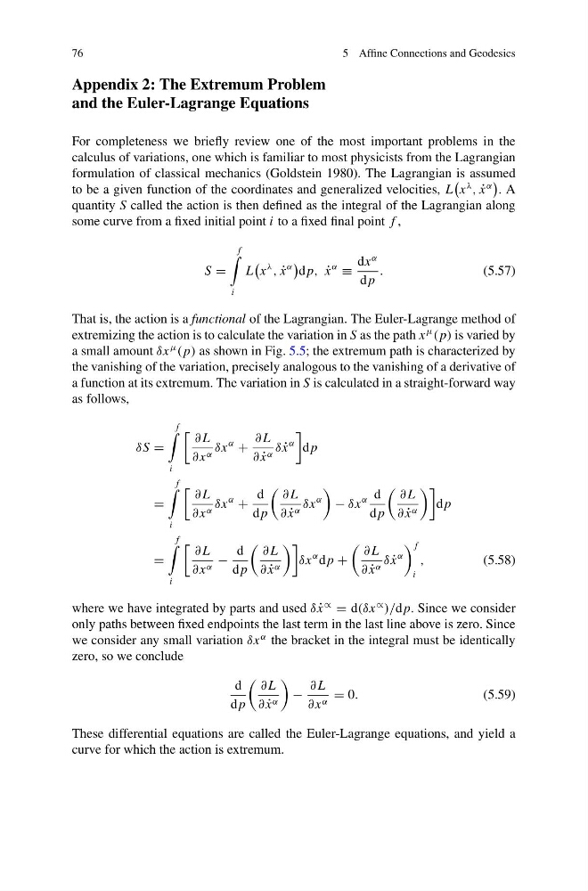
That is, the action is a functional of the Lagrangian. The Euler-Lagrange method of
extremizing the action is to calculate the variation in S as the path x
μ
( p) is varied by
a small amount δx
μ
( p) as shown in Fig. 5.5; the extremum path is characterized by
the vanishing of the variation, precisely analogous to the vanishing of a derivative of
a function at its extremum. The variation in S is calculated in a straight-forward way
as follows,
δS =
f
i
∂ L
∂ x α δx
α
+
∂ L
∂ ˙
x α δ ˙
x
α
d p
=
f
i
∂ L
∂ x α δx
α
+
d
d p
∂ L
∂ ˙
x α δx
α
− δx
α d
d p
∂ L
∂ ˙
x α
d p
=
f
i
∂ L
∂ x α −
d
d p
∂ L
∂ ˙
x α
δx
α d p +
∂ L
∂ ˙
x α δ ˙
x
α
f
i
,
(5.58)
where we have integrated by parts and used δ ˙
x
∝
= d(δx
∝
)/d p. Since we consider
only paths between fixed endpoints the last term in the last line above is zero. Since
we consider any small variation δx
α the bracket in the integral must be identically
zero, so we conclude
d
d p
∂ L
∂ ˙
x α
−
∂ L
∂ x α = 0.
(5.59)
These differential equations are called the Euler-Lagrange equations, and yield a
curve for which the action is extremum.
5 Affine Connections and Geodesics
Appendix 2: The Extremum Problem
and the Euler-Lagrange Equations
For completeness we briefly review one of the most important problems in the
calculus of variations, one which is familiar to most physicists from the Lagrangian
formulation of classical mechanics (Goldstein 1980). The Lagrangian is assumed
to be a given function of the coordinates and generalized velocities, L
x
λ
, ˙
x
α
. A
quantity S called the action is then defined as the integral of the Lagrangian along
some curve from a fixed initial point i to a fixed final point f ,
S =
f
i
L
x
λ
, ˙
x
α
d p, ˙
x
α
≡
dx
α
d p
.
(5.57)
That is, the action is a functional of the Lagrangian. The Euler-Lagrange method of
extremizing the action is to calculate the variation in S as the path x
μ
( p) is varied by
a small amount δx
μ
( p) as shown in Fig. 5.5; the extremum path is characterized by
the vanishing of the variation, precisely analogous to the vanishing of a derivative of
a function at its extremum. The variation in S is calculated in a straight-forward way
as follows,
δS =
f
i
∂ L
∂ x α δx
α
+
∂ L
∂ ˙
x α δ ˙
x
α
d p
=
f
i
∂ L
∂ x α δx
α
+
d
d p
∂ L
∂ ˙
x α δx
α
− δx
α d
d p
∂ L
∂ ˙
x α
d p
=
f
i
∂ L
∂ x α −
d
d p
∂ L
∂ ˙
x α
δx
α d p +
∂ L
∂ ˙
x α δ ˙
x
α
f
i
,
(5.58)
where we have integrated by parts and used δ ˙
x
∝
= d(δx
∝
)/d p. Since we consider
only paths between fixed endpoints the last term in the last line above is zero. Since
we consider any small variation δx
α the bracket in the integral must be identically
zero, so we conclude
d
d p
∂ L
∂ ˙
x α
−
∂ L
∂ x α = 0.
(5.59)
These differential equations are called the Euler-Lagrange equations, and yield a
curve for which the action is extremum.