

70
5 Affine Connections and Geodesics
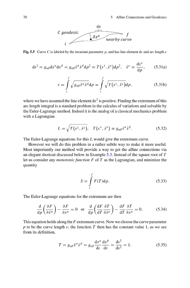
Fig. 5.5 Curve C is labeled by the invariant parameter p, and has line element ds and arc length s
ds
2
= g αβ dx
α dx
β
= g αβ ˙
x
α
˙
x
β d p
2
≡ T
x
λ
, ˙
x
κ
d p
2
, ˙
x
κ
≡
dx
κ
d p
,
(5.31a)
s =
f
i
g αβ ˙
x α ˙
x β d p =
f
i
T
x λ , ˙
x κ
d p,
(5.31b)
where we have assumed the line element ds
2 is positive. Finding the extremum of this
arc length integral is a standard problem in the calculus of variations and solvable by
the Euler-Lagrange method. Indeed it is the analog of a classical mechanics problem
with a Lagrangian
L =
T
x λ , ˙
x κ
, T
x
λ
, ˙
x
κ
≡ g αβ ˙
x
α
˙
x
β
.
(5.32)
The Euler-Lagrange equations for this L would give the extremum curve.
However we will do this problem in a rather subtle way to make it more useful.
Most importantly our method will provide a way to get the affine connections via
an elegant shortcut discussed below in Example 5.3. Instead of the square root of T
let us consider any monotonic function F of T as the Lagrangian, and minimize the
quantity
S =
f
i
F(T )d p.
(5.33)
The Euler-Lagrange equations for the extremum are then
d
d p
∂ F
∂ ˙
x α
−
∂ F
∂ x α = 0 or
d
d p
dF
dT
∂ T
∂ ˙
x α
−
dF
dT
∂ T
∂ x α = 0.
(5.34)
This equation holds along the F extremum curve. Now we choose the curve parameter
p to be the curve length s; the function T then has the constant value 1, as we see
from its definition,
T = g αβ ˙
x
α
˙
x
β
= g αβ
dx
α
ds
dx
β
ds
=
ds
2
ds 2 = 1.
(5.35)
5 Affine Connections and Geodesics
Fig. 5.5 Curve C is labeled by the invariant parameter p, and has line element ds and arc length s
ds
2
= g αβ dx
α dx
β
= g αβ ˙
x
α
˙
x
β d p
2
≡ T
x
λ
, ˙
x
κ
d p
2
, ˙
x
κ
≡
dx
κ
d p
,
(5.31a)
s =
f
i
g αβ ˙
x α ˙
x β d p =
f
i
T
x λ , ˙
x κ
d p,
(5.31b)
where we have assumed the line element ds
2 is positive. Finding the extremum of this
arc length integral is a standard problem in the calculus of variations and solvable by
the Euler-Lagrange method. Indeed it is the analog of a classical mechanics problem
with a Lagrangian
L =
T
x λ , ˙
x κ
, T
x
λ
, ˙
x
κ
≡ g αβ ˙
x
α
˙
x
β
.
(5.32)
The Euler-Lagrange equations for this L would give the extremum curve.
However we will do this problem in a rather subtle way to make it more useful.
Most importantly our method will provide a way to get the affine connections via
an elegant shortcut discussed below in Example 5.3. Instead of the square root of T
let us consider any monotonic function F of T as the Lagrangian, and minimize the
quantity
S =
f
i
F(T )d p.
(5.33)
The Euler-Lagrange equations for the extremum are then
d
d p
∂ F
∂ ˙
x α
−
∂ F
∂ x α = 0 or
d
d p
dF
dT
∂ T
∂ ˙
x α
−
dF
dT
∂ T
∂ x α = 0.
(5.34)
This equation holds along the F extremum curve. Now we choose the curve parameter
p to be the curve length s; the function T then has the constant value 1, as we see
from its definition,
T = g αβ ˙
x
α
˙
x
β
= g αβ
dx
α
ds
dx
β
ds
=
ds
2
ds 2 = 1.
(5.35)