

5.3 Parallel Displacement
65
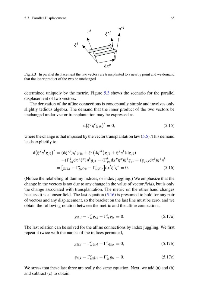
Fig. 5.3 In parallel displacement the two vectors are transplanted to a nearby point and we demand
that the inner product of the two be unchanged
determined uniquely by the metric. Figure 5.3 shows the scenario for the parallel
displacement of two vectors.
The derivation of the affine connections is conceptually simple and involves only
slightly tedious algebra. The demand that the inner product of the two vectors be
unchanged under vector transplantation may be expressed as
d
ξ
j
η
k g jk
∗ = 0,
(5.15)
where the change is that imposed by the vector transplantation law (5.5). This demand
leads explicitly to
d
ξ
j
η
k g jk
∗ = (dξ
∗ j
)η
k g jk + ξ
j
dη
∗k
g jk + ξ
j
η
k
(dg jk )
= −((
j
pq dx
p
ξ
q
)η
k g jk − ((
k
pq dx
p
η
q
)ξ
j g jk + (g jk,l dx
l
)ξ
j
η
k
=
g ik,l −
r
li g rk −
r
lk g ir
dx
l
ξ
i
η
k
= 0.
(5.16)
(Notice the relabeling of dummy indices, or index juggling.) We emphasize that the
change in the vectors is not due to any change in the value of vector fields, but is only
the change associated with transplantation. The metric on the other hand changes
because it is a tensor field. The last equation (5.16) is presumed to hold for any pair
of vectors and any displacement, so the bracket on the last line must be zero, and we
obtain the following relation between the metric and the affine connections,
g ik,l −
r
li g rk −
r
lk g ir = 0.
(5.17a)
The last relation can be solved for the affine connections by index juggling. We first
repeat it twice with the names of the indices permuted,
g kl,i −
r
ik g rl −
r
il g kr = 0,
(5.17b)
g li,k −
r
kl g ri −
r
ki g lr = 0.
(5.17c)
We stress that these last three are really the same equation. Next, we add (a) and (b)
and subtract (c) to obtain
65
Fig. 5.3 In parallel displacement the two vectors are transplanted to a nearby point and we demand
that the inner product of the two be unchanged
determined uniquely by the metric. Figure 5.3 shows the scenario for the parallel
displacement of two vectors.
The derivation of the affine connections is conceptually simple and involves only
slightly tedious algebra. The demand that the inner product of the two vectors be
unchanged under vector transplantation may be expressed as
d
ξ
j
η
k g jk
∗ = 0,
(5.15)
where the change is that imposed by the vector transplantation law (5.5). This demand
leads explicitly to
d
ξ
j
η
k g jk
∗ = (dξ
∗ j
)η
k g jk + ξ
j
dη
∗k
g jk + ξ
j
η
k
(dg jk )
= −((
j
pq dx
p
ξ
q
)η
k g jk − ((
k
pq dx
p
η
q
)ξ
j g jk + (g jk,l dx
l
)ξ
j
η
k
=
g ik,l −
r
li g rk −
r
lk g ir
dx
l
ξ
i
η
k
= 0.
(5.16)
(Notice the relabeling of dummy indices, or index juggling.) We emphasize that the
change in the vectors is not due to any change in the value of vector fields, but is only
the change associated with transplantation. The metric on the other hand changes
because it is a tensor field. The last equation (5.16) is presumed to hold for any pair
of vectors and any displacement, so the bracket on the last line must be zero, and we
obtain the following relation between the metric and the affine connections,
g ik,l −
r
li g rk −
r
lk g ir = 0.
(5.17a)
The last relation can be solved for the affine connections by index juggling. We first
repeat it twice with the names of the indices permuted,
g kl,i −
r
ik g rl −
r
il g kr = 0,
(5.17b)
g li,k −
r
kl g ri −
r
ki g lr = 0.
(5.17c)
We stress that these last three are really the same equation. Next, we add (a) and (b)
and subtract (c) to obtain