

Appendix 3: Electromagnetic Wave Sources
187
Appendix 3: Electromagnetic Wave Sources
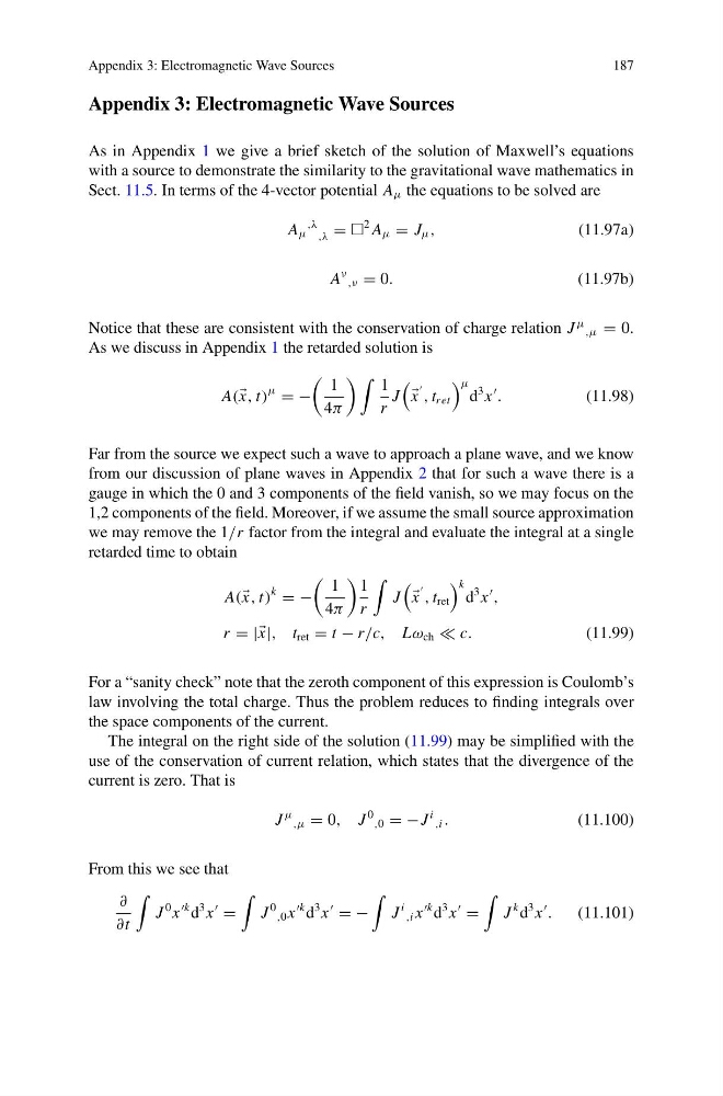
As in Appendix 1 we give a brief sketch of the solution of Maxwell’s equations
with a source to demonstrate the similarity to the gravitational wave mathematics in
Sect. 11.5. In terms of the 4-vector potential A μ the equations to be solved are
A μ
,λ
,λ =
2 A μ = J μ ,
(11.97a)
A
ν ,ν = 0.
(11.97b)
Notice that these are consistent with the conservation of charge relation J
μ ,μ = 0.
As we discuss in Appendix 1 the retarded solution is
A( x, t)
μ = −
1
4π
1
r
J
x
, t ret
μ
d
3 x
.
(11.98)
Far from the source we expect such a wave to approach a plane wave, and we know
from our discussion of plane waves in Appendix 2 that for such a wave there is a
gauge in which the 0 and 3 components of the field vanish, so we may focus on the
1,2 components of the field. Moreover, if we assume the small source approximation
we may remove the 1/r factor from the integral and evaluate the integral at a single
retarded time to obtain
A( x, t)
k = −
1
4π
1
r
J
x
, t ret
k
d
3 x
,
r = | x|, t ret = t − r/c, Lω ch c.
(11.99)
For a “sanity check” note that the zeroth component of this expression is Coulomb’s
law involving the total charge. Thus the problem reduces to finding integrals over
the space components of the current.
The integral on the right side of the solution (11.99) may be simplified with the
use of the conservation of current relation, which states that the divergence of the
current is zero. That is
J
μ ,μ = 0, J
0 ,0 = −J
i ,i .
(11.100)
From this we see that
∂
∂t
J
0 x
k d
3 x
=
J
0 ,0 x
k d
3 x
= −
J
i ,i x
k d
3 x
=
J
k d
3 x
.
(11.101)
187
Appendix 3: Electromagnetic Wave Sources
As in Appendix 1 we give a brief sketch of the solution of Maxwell’s equations
with a source to demonstrate the similarity to the gravitational wave mathematics in
Sect. 11.5. In terms of the 4-vector potential A μ the equations to be solved are
A μ
,λ
,λ =
2 A μ = J μ ,
(11.97a)
A
ν ,ν = 0.
(11.97b)
Notice that these are consistent with the conservation of charge relation J
μ ,μ = 0.
As we discuss in Appendix 1 the retarded solution is
A( x, t)
μ = −
1
4π
1
r
J
x
, t ret
μ
d
3 x
.
(11.98)
Far from the source we expect such a wave to approach a plane wave, and we know
from our discussion of plane waves in Appendix 2 that for such a wave there is a
gauge in which the 0 and 3 components of the field vanish, so we may focus on the
1,2 components of the field. Moreover, if we assume the small source approximation
we may remove the 1/r factor from the integral and evaluate the integral at a single
retarded time to obtain
A( x, t)
k = −
1
4π
1
r
J
x
, t ret
k
d
3 x
,
r = | x|, t ret = t − r/c, Lω ch c.
(11.99)
For a “sanity check” note that the zeroth component of this expression is Coulomb’s
law involving the total charge. Thus the problem reduces to finding integrals over
the space components of the current.
The integral on the right side of the solution (11.99) may be simplified with the
use of the conservation of current relation, which states that the divergence of the
current is zero. That is
J
μ ,μ = 0, J
0 ,0 = −J
i ,i .
(11.100)
From this we see that
∂
∂t
J
0 x
k d
3 x
=
J
0 ,0 x
k d
3 x
= −
J
i ,i x
k d
3 x
=
J
k d
3 x
.
(11.101)