

9 Mössbauer Spectroscopic Studies on Atomic Diffusion in Materials
485
This model corresponds to a set of the reaction kinetic equations described above.
We now try to reproduce the whole changes observed in the spectra up to 1000 K. We
simulate the kinetic equations of the interstitial C I
Fe and the substitutional C S
Fe
=
(1−C I
Fe ) reacting with vacancies C V and self-interstitials C I which arises from the
above mentioned “diffusion–reaction”. Here, K1, K2, K3, and K4 are the reaction
coefficients.
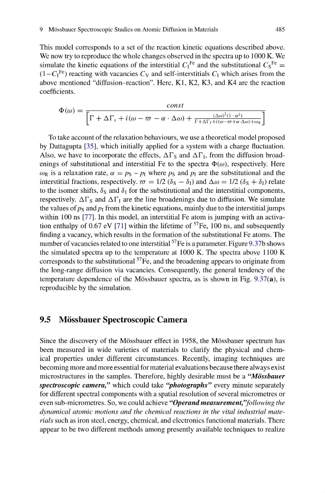
=
const
+ s + i(ω − − α · +
((ω)
2 (1−α 2 )
+ I +i(ω− +α·ω)+ω R
To take account of the relaxation behaviours, we use a theoretical model proposed
by Dattagupta [35], which initially applied for a system with a charge fluctuation.
Also, we have to incorporate the effects, S and I , from the diffusion broadenings of substitutional and interstitial Fe to the spectra (ω), respectively. Here
ω R is a relaxation rate, α = p S – p I where p S and p I are the substitutional and the
interstitial fractions, respectively. = 1/2 (δ S − δ I ) and ω = 1/2 (δ S + δ I ) relate
to the isomer shifts, δ S and δ I for the substitutional and the interstitial components,
respectively. S and I are the line broadenings due to diffusion. We simulate
the values of p S and p I from the kinetic equations, mainly due to the interstitial jumps
within 100 ns [77]. In this model, an interstitial Fe atom is jumping with an activation enthalpy of 0.67 eV [71] within the lifetime of
57 Fe, 100 ns, and subsequently
finding a vacancy, which results in the formation of the substitutional Fe atoms. The
number of vacancies related to one interstitial
57 Fe is a parameter. Figure 9.37b shows
the simulated spectra up to the temperature at 1000 K. The spectra above 1100 K
corresponds to the substitutional
57 Fe, and the broadening appears to originate from
the long-range diffusion via vacancies. Consequently, the general tendency of the
temperature dependence of the Mössbauer spectra, as is shown in Fig. 9.37(a), is
reproducible by the simulation.
9.5 Mössbauer Spectroscopic Camera
Since the discovery of the Mössbauer effect in 1958, the Mössbauer spectrum has
been measured in wide varieties of materials to clarify the physical and chemical properties under different circumstances. Recently, imaging techniques are
becoming more and more essential for material evaluations because there always exist
microstructures in the samples. Therefore, highly desirable must be a “Mössbauer
spectroscopic camera,” which could take “photographs” every minute separately
for different spectral components with a spatial resolution of several micrometres or
even sub-micrometres. So, we could achieve “Operand measurement,”following the
dynamical atomic motions and the chemical reactions in the vital industrial materials such as iron steel, energy, chemical, and electronics functional materials. There
appear to be two different methods among presently available techniques to realize
485
This model corresponds to a set of the reaction kinetic equations described above.
We now try to reproduce the whole changes observed in the spectra up to 1000 K. We
simulate the kinetic equations of the interstitial C I
Fe and the substitutional C S
Fe
=
(1−C I
Fe ) reacting with vacancies C V and self-interstitials C I which arises from the
above mentioned “diffusion–reaction”. Here, K1, K2, K3, and K4 are the reaction
coefficients.
=
const
+ s + i(ω − − α · +
((ω)
2 (1−α 2 )
+ I +i(ω− +α·ω)+ω R
To take account of the relaxation behaviours, we use a theoretical model proposed
by Dattagupta [35], which initially applied for a system with a charge fluctuation.
Also, we have to incorporate the effects, S and I , from the diffusion broadenings of substitutional and interstitial Fe to the spectra (ω), respectively. Here
ω R is a relaxation rate, α = p S – p I where p S and p I are the substitutional and the
interstitial fractions, respectively. = 1/2 (δ S − δ I ) and ω = 1/2 (δ S + δ I ) relate
to the isomer shifts, δ S and δ I for the substitutional and the interstitial components,
respectively. S and I are the line broadenings due to diffusion. We simulate
the values of p S and p I from the kinetic equations, mainly due to the interstitial jumps
within 100 ns [77]. In this model, an interstitial Fe atom is jumping with an activation enthalpy of 0.67 eV [71] within the lifetime of
57 Fe, 100 ns, and subsequently
finding a vacancy, which results in the formation of the substitutional Fe atoms. The
number of vacancies related to one interstitial
57 Fe is a parameter. Figure 9.37b shows
the simulated spectra up to the temperature at 1000 K. The spectra above 1100 K
corresponds to the substitutional
57 Fe, and the broadening appears to originate from
the long-range diffusion via vacancies. Consequently, the general tendency of the
temperature dependence of the Mössbauer spectra, as is shown in Fig. 9.37(a), is
reproducible by the simulation.
9.5 Mössbauer Spectroscopic Camera
Since the discovery of the Mössbauer effect in 1958, the Mössbauer spectrum has
been measured in wide varieties of materials to clarify the physical and chemical properties under different circumstances. Recently, imaging techniques are
becoming more and more essential for material evaluations because there always exist
microstructures in the samples. Therefore, highly desirable must be a “Mössbauer
spectroscopic camera,” which could take “photographs” every minute separately
for different spectral components with a spatial resolution of several micrometres or
even sub-micrometres. So, we could achieve “Operand measurement,”following the
dynamical atomic motions and the chemical reactions in the vital industrial materials such as iron steel, energy, chemical, and electronics functional materials. There
appear to be two different methods among presently available techniques to realize