

4 From Small Molecules to Complex Systems: A Survey of Chemical …
187
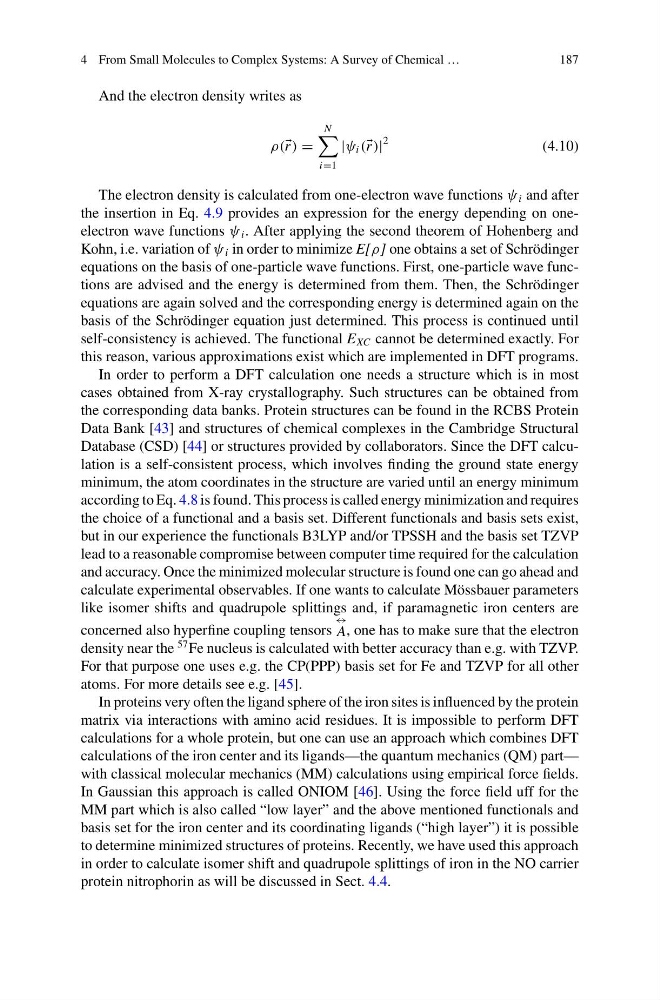
And the electron density writes as
ρ( r ) =
N
i=1
|ψ i ( r )|
2
(4.10)
The electron density is calculated from one-electron wave functions ψ i and after
the insertion in Eq. 4.9 provides an expression for the energy depending on oneelectron wave functions ψ i . After applying the second theorem of Hohenberg and
Kohn, i.e. variation of ψ i in order to minimize E[ρ] one obtains a set of Schrödinger
equations on the basis of one-particle wave functions. First, one-particle wave functions are advised and the energy is determined from them. Then, the Schrödinger
equations are again solved and the corresponding energy is determined again on the
basis of the Schrödinger equation just determined. This process is continued until
self-consistency is achieved. The functional E XC cannot be determined exactly. For
this reason, various approximations exist which are implemented in DFT programs.
In order to perform a DFT calculation one needs a structure which is in most
cases obtained from X-ray crystallography. Such structures can be obtained from
the corresponding data banks. Protein structures can be found in the RCBS Protein
Data Bank [43] and structures of chemical complexes in the Cambridge Structural
Database (CSD) [44] or structures provided by collaborators. Since the DFT calculation is a self-consistent process, which involves finding the ground state energy
minimum, the atom coordinates in the structure are varied until an energy minimum
according to Eq. 4.8 is found. This process is called energy minimization and requires
the choice of a functional and a basis set. Different functionals and basis sets exist,
but in our experience the functionals B3LYP and/or TPSSH and the basis set TZVP
lead to a reasonable compromise between computer time required for the calculation
and accuracy. Once the minimized molecular structure is found one can go ahead and
calculate experimental observables. If one wants to calculate Mössbauer parameters
like isomer shifts and quadrupole splittings and, if paramagnetic iron centers are
concerned also hyperfine coupling tensors
↔
A, one has to make sure that the electron
density near the
57 Fe nucleus is calculated with better accuracy than e.g. with TZVP.
For that purpose one uses e.g. the CP(PPP) basis set for Fe and TZVP for all other
atoms. For more details see e.g. [45].
In proteins very often the ligand sphere of the iron sites is influenced by the protein
matrix via interactions with amino acid residues. It is impossible to perform DFT
calculations for a whole protein, but one can use an approach which combines DFT
calculations of the iron center and its ligands—the quantum mechanics (QM) part—
with classical molecular mechanics (MM) calculations using empirical force fields.
In Gaussian this approach is called ONIOM [46]. Using the force field uff for the
MM part which is also called “low layer” and the above mentioned functionals and
basis set for the iron center and its coordinating ligands (“high layer”) it is possible
to determine minimized structures of proteins. Recently, we have used this approach
in order to calculate isomer shift and quadrupole splittings of iron in the NO carrier
protein nitrophorin as will be discussed in Sect. 4.4.
187
And the electron density writes as
ρ( r ) =
N
i=1
|ψ i ( r )|
2
(4.10)
The electron density is calculated from one-electron wave functions ψ i and after
the insertion in Eq. 4.9 provides an expression for the energy depending on oneelectron wave functions ψ i . After applying the second theorem of Hohenberg and
Kohn, i.e. variation of ψ i in order to minimize E[ρ] one obtains a set of Schrödinger
equations on the basis of one-particle wave functions. First, one-particle wave functions are advised and the energy is determined from them. Then, the Schrödinger
equations are again solved and the corresponding energy is determined again on the
basis of the Schrödinger equation just determined. This process is continued until
self-consistency is achieved. The functional E XC cannot be determined exactly. For
this reason, various approximations exist which are implemented in DFT programs.
In order to perform a DFT calculation one needs a structure which is in most
cases obtained from X-ray crystallography. Such structures can be obtained from
the corresponding data banks. Protein structures can be found in the RCBS Protein
Data Bank [43] and structures of chemical complexes in the Cambridge Structural
Database (CSD) [44] or structures provided by collaborators. Since the DFT calculation is a self-consistent process, which involves finding the ground state energy
minimum, the atom coordinates in the structure are varied until an energy minimum
according to Eq. 4.8 is found. This process is called energy minimization and requires
the choice of a functional and a basis set. Different functionals and basis sets exist,
but in our experience the functionals B3LYP and/or TPSSH and the basis set TZVP
lead to a reasonable compromise between computer time required for the calculation
and accuracy. Once the minimized molecular structure is found one can go ahead and
calculate experimental observables. If one wants to calculate Mössbauer parameters
like isomer shifts and quadrupole splittings and, if paramagnetic iron centers are
concerned also hyperfine coupling tensors
↔
A, one has to make sure that the electron
density near the
57 Fe nucleus is calculated with better accuracy than e.g. with TZVP.
For that purpose one uses e.g. the CP(PPP) basis set for Fe and TZVP for all other
atoms. For more details see e.g. [45].
In proteins very often the ligand sphere of the iron sites is influenced by the protein
matrix via interactions with amino acid residues. It is impossible to perform DFT
calculations for a whole protein, but one can use an approach which combines DFT
calculations of the iron center and its ligands—the quantum mechanics (QM) part—
with classical molecular mechanics (MM) calculations using empirical force fields.
In Gaussian this approach is called ONIOM [46]. Using the force field uff for the
MM part which is also called “low layer” and the above mentioned functionals and
basis set for the iron center and its coordinating ligands (“high layer”) it is possible
to determine minimized structures of proteins. Recently, we have used this approach
in order to calculate isomer shift and quadrupole splittings of iron in the NO carrier
protein nitrophorin as will be discussed in Sect. 4.4.