

186
V. Schünemann
varying the Euler angles of the molecular axes with respect to the laboratory frame
given by the direction of the external field and the direction of the γ-ray. Details of
this procedure can be found in the classic work of Münck et al. [38].
4.2.4 Calculation of Mössbauer Parameters with Quantum
Chemical Methods
Nowadays Mössbauer parameters for iron molecules can be calculated using theoretical models based on density functional theory (DFT). These calculations do not
necessarily need to be performed by quantum chemists. Using the software packages ORCA [39], Gaussian [40] and/or Turbomole [41] it is possible also for the
spectroscopist to achieve reasonable results. After the installation of these software
packages the user can choose suitable models to perform calculations without further
major programming skills.
DFT represents a possibility to solve the many-particle Schrödinger equation
of complex molecules numerically. It is important to note that the central quantum
mechanical observable of DFT is the ground state electron density ρ 0 . The theoretical
basis of DFT is given by two theorems formulated by Hohenberg and Kohn [42].
The first states that every system of interacting electrons in an external potential is
determined by its electron density ρ 0 . Thus, the ground state energy is also determined
by the density ρ 0 , in other words, the electronic ground state energy E is a function
of ρ 0 and a functional exists of the form:
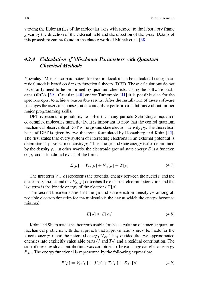
E[ρ] = V ne [ρ] + V ee [ρ] + T [ρ]
(4.7)
The first term V ne [ρ] represents the potential energy between the nuclei n and the
electrons e, the second one V ee [ρ] describes the electron–electron interaction and the
last term is the kinetic energy of the electrons T [ρ].
The second theorem states that the ground state electron density ρ 0 among all
possible electron densities for the molecule is the one at which the energy becomes
minimal:
E[ρ] ≥ E[ρ 0 ]
(4.8)
Kohn and Sham made the theorems usable for the calculation of concrete quantum
mechanical problems with the approach that approximations must be made for the
kinetic energy T and the potential energy V ee . They divided the two approximated
energies into explicitly calculable parts (J and T S ) and a residual contribution. The
sum of these residual contributions was combined to the exchange correlation energy
E XC . The energy functional is represented by the following expression:
E[ρ] = V ne [ρ] + J [ρ] + T S [ρ] + E XC [ρ]
(4.9)
V. Schünemann
varying the Euler angles of the molecular axes with respect to the laboratory frame
given by the direction of the external field and the direction of the γ-ray. Details of
this procedure can be found in the classic work of Münck et al. [38].
4.2.4 Calculation of Mössbauer Parameters with Quantum
Chemical Methods
Nowadays Mössbauer parameters for iron molecules can be calculated using theoretical models based on density functional theory (DFT). These calculations do not
necessarily need to be performed by quantum chemists. Using the software packages ORCA [39], Gaussian [40] and/or Turbomole [41] it is possible also for the
spectroscopist to achieve reasonable results. After the installation of these software
packages the user can choose suitable models to perform calculations without further
major programming skills.
DFT represents a possibility to solve the many-particle Schrödinger equation
of complex molecules numerically. It is important to note that the central quantum
mechanical observable of DFT is the ground state electron density ρ 0 . The theoretical
basis of DFT is given by two theorems formulated by Hohenberg and Kohn [42].
The first states that every system of interacting electrons in an external potential is
determined by its electron density ρ 0 . Thus, the ground state energy is also determined
by the density ρ 0 , in other words, the electronic ground state energy E is a function
of ρ 0 and a functional exists of the form:
E[ρ] = V ne [ρ] + V ee [ρ] + T [ρ]
(4.7)
The first term V ne [ρ] represents the potential energy between the nuclei n and the
electrons e, the second one V ee [ρ] describes the electron–electron interaction and the
last term is the kinetic energy of the electrons T [ρ].
The second theorem states that the ground state electron density ρ 0 among all
possible electron densities for the molecule is the one at which the energy becomes
minimal:
E[ρ] ≥ E[ρ 0 ]
(4.8)
Kohn and Sham made the theorems usable for the calculation of concrete quantum
mechanical problems with the approach that approximations must be made for the
kinetic energy T and the potential energy V ee . They divided the two approximated
energies into explicitly calculable parts (J and T S ) and a residual contribution. The
sum of these residual contributions was combined to the exchange correlation energy
E XC . The energy functional is represented by the following expression:
E[ρ] = V ne [ρ] + J [ρ] + T S [ρ] + E XC [ρ]
(4.9)