

182
V. Schünemann
runs from −S; −S + 1;…S − 1; S. The spin-orbit interaction of the paramagnetic
iron ion manifests itself in the spin Hamiltonian concept in two parameters, the zero
field splitting D and the rhombicity parameter E/D since the orbital momentum in 3d
transition metals is nearly quenched. In ions which exert a ligand field, caused by the
negative charge of the surrounding ligands like in chemical complexes (s. Figure 4.1)
the orbital momentum is not totally quenched and can be treated as a second order
effect. This leads to an energy splitting of the |S; m s > states even in zero magnetic
fields. These energy splittings due to zero field splitting are quite small, normally in
the order of some Kelvin.
The coupling of the total orbital momentum
− →
L to the total spin momentum
− →
S
can be treated via perturbation theory. This concept was first introduced in order to
describe electron paramagnetic resonance (EPR) signals of paramagnetic ions [32]
and was later applied to paramagnetic Mössbauer spectroscopy by Wickmann et al.
[33]. A paramagnetic iron with spin quantum number S in a ligand field is than
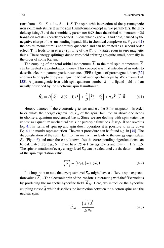
usually described by the electronic spin Hamiltonian:
ˆ
H S = D
ˆ
S
2
z − S(S + 1)/3
+
E
D
ˆ
S
2
x − ˆ
S
2
y
+ μ B
S ·
↔
g ·
B
(4.1)
Hereby denotes
↔
g the electronic g-tensor and μ B the Bohr magneton. In order
to calculate the energy eigenvalues E S of the spin Hamiltonian above one needs
to choose a quantum mechanical basis. Since we are dealing with spin states we
choose as a quantum mechanical basis the pure spin functions |S; m s >. If one rewrites
Eq. 4.1 in terms of spin up and spin down operators it is possible to write down
Eq. 4.1 in matrix representation. The exact procedure can be found e.g. in [34]. The
diagonalization of the spin Hamiltonian matrix than leads to the energy eigenvalues
E si (Fig. 4.6) and once these are known also the corresponding eigenfunctions can
be calculated. For e.g., S = 2 we have 2S + 1 energy levels and thus i = 1, 2, ...,5.
The spin orientation of every energy level E si can be calculated via the determination
of the spin expectation value.
− →
S
=
S x ,
S y
, S z
(4.2)
It is important to note that every sublevel E Si might have a different spin expectation value
− →
S i . The electronic spin of the iron ion is interacting with the
57 Fe nucleus
by producing the magnetic hyperfine field
− →
B hf . Here, we introduce the hyperfine
coupling tensor
↔
A which describes the interaction between the electron spins and the
nuclear spin:
− →
B h f =
− →
S
← →
A
g n μ n
(4.3)
V. Schünemann
runs from −S; −S + 1;…S − 1; S. The spin-orbit interaction of the paramagnetic
iron ion manifests itself in the spin Hamiltonian concept in two parameters, the zero
field splitting D and the rhombicity parameter E/D since the orbital momentum in 3d
transition metals is nearly quenched. In ions which exert a ligand field, caused by the
negative charge of the surrounding ligands like in chemical complexes (s. Figure 4.1)
the orbital momentum is not totally quenched and can be treated as a second order
effect. This leads to an energy splitting of the |S; m s > states even in zero magnetic
fields. These energy splittings due to zero field splitting are quite small, normally in
the order of some Kelvin.
The coupling of the total orbital momentum
− →
L to the total spin momentum
− →
S
can be treated via perturbation theory. This concept was first introduced in order to
describe electron paramagnetic resonance (EPR) signals of paramagnetic ions [32]
and was later applied to paramagnetic Mössbauer spectroscopy by Wickmann et al.
[33]. A paramagnetic iron with spin quantum number S in a ligand field is than
usually described by the electronic spin Hamiltonian:
ˆ
H S = D
ˆ
S
2
z − S(S + 1)/3
+
E
D
ˆ
S
2
x − ˆ
S
2
y
+ μ B
S ·
↔
g ·
B
(4.1)
Hereby denotes
↔
g the electronic g-tensor and μ B the Bohr magneton. In order
to calculate the energy eigenvalues E S of the spin Hamiltonian above one needs
to choose a quantum mechanical basis. Since we are dealing with spin states we
choose as a quantum mechanical basis the pure spin functions |S; m s >. If one rewrites
Eq. 4.1 in terms of spin up and spin down operators it is possible to write down
Eq. 4.1 in matrix representation. The exact procedure can be found e.g. in [34]. The
diagonalization of the spin Hamiltonian matrix than leads to the energy eigenvalues
E si (Fig. 4.6) and once these are known also the corresponding eigenfunctions can
be calculated. For e.g., S = 2 we have 2S + 1 energy levels and thus i = 1, 2, ...,5.
The spin orientation of every energy level E si can be calculated via the determination
of the spin expectation value.
− →
S
=
S x ,
S y
, S z
(4.2)
It is important to note that every sublevel E Si might have a different spin expectation value
− →
S i . The electronic spin of the iron ion is interacting with the
57 Fe nucleus
by producing the magnetic hyperfine field
− →
B hf . Here, we introduce the hyperfine
coupling tensor
↔
A which describes the interaction between the electron spins and the
nuclear spin:
− →
B h f =
− →
S
← →
A
g n μ n
(4.3)