

2 Synchrotron-Radiation-Based Energy-Domain Mössbauer …
97
The experimental time spectrum is ¯
I exp (q, t) = ¯
I (q, t) ⊗ D(t) + B. The γ-rays
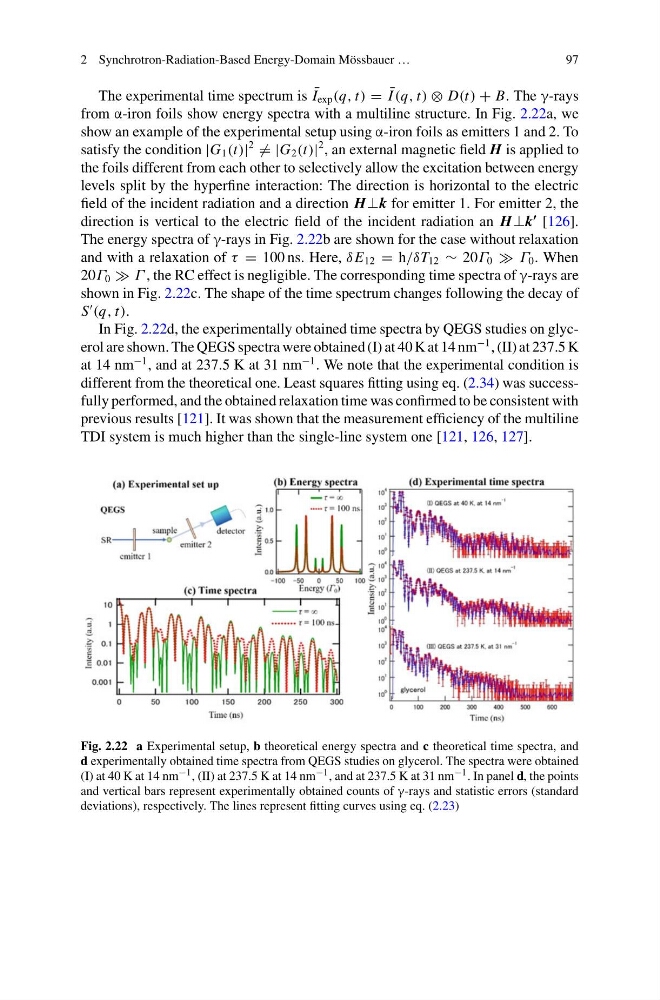
from α-iron foils show energy spectra with a multiline structure. In Fig. 2.22a, we
show an example of the experimental setup using α-iron foils as emitters 1 and 2. To
satisfy the condition |G 1 (t)|
2
= |G 2 (t)|
2 , an external magnetic field H is applied to
the foils different from each other to selectively allow the excitation between energy
levels split by the hyperfine interaction: The direction is horizontal to the electric
field of the incident radiation and a direction H⊥k for emitter 1. For emitter 2, the
direction is vertical to the electric field of the incident radiation an H⊥k
[126].
The energy spectra of γ-rays in Fig. 2.22b are shown for the case without relaxation
and with a relaxation of τ = 100 ns. Here, δ E 12 = h/δT 12 ∼ 20Γ 0 Γ 0 . When
20Γ 0 Γ , the RC effect is negligible. The corresponding time spectra of γ-rays are
shown in Fig. 2.22c. The shape of the time spectrum changes following the decay of
S
(q, t).
In Fig. 2.22d, the experimentally obtained time spectra by QEGS studies on glycerol are shown. The QEGS spectra were obtained (I) at 40 K at 14 nm
−1 , (II) at 237.5 K
at 14 nm
−1 , and at 237.5 K at 31 nm
−1 . We note that the experimental condition is
different from the theoretical one. Least squares fitting using eq. (2.34) was successfully performed, and the obtained relaxation time was confirmed to be consistent with
previous results [121]. It was shown that the measurement efficiency of the multiline
TDI system is much higher than the single-line system one [121, 126, 127].
Fig. 2.22 a Experimental setup, b theoretical energy spectra and c theoretical time spectra, and
d experimentally obtained time spectra from QEGS studies on glycerol. The spectra were obtained
(I) at 40 K at 14 nm −1 , (II) at 237.5 K at 14 nm −1 , and at 237.5 K at 31 nm −1 . In panel d, the points
and vertical bars represent experimentally obtained counts of γ-rays and statistic errors (standard
deviations), respectively. The lines represent fitting curves using eq. (2.23)
97
The experimental time spectrum is ¯
I exp (q, t) = ¯
I (q, t) ⊗ D(t) + B. The γ-rays
from α-iron foils show energy spectra with a multiline structure. In Fig. 2.22a, we
show an example of the experimental setup using α-iron foils as emitters 1 and 2. To
satisfy the condition |G 1 (t)|
2
= |G 2 (t)|
2 , an external magnetic field H is applied to
the foils different from each other to selectively allow the excitation between energy
levels split by the hyperfine interaction: The direction is horizontal to the electric
field of the incident radiation and a direction H⊥k for emitter 1. For emitter 2, the
direction is vertical to the electric field of the incident radiation an H⊥k
[126].
The energy spectra of γ-rays in Fig. 2.22b are shown for the case without relaxation
and with a relaxation of τ = 100 ns. Here, δ E 12 = h/δT 12 ∼ 20Γ 0 Γ 0 . When
20Γ 0 Γ , the RC effect is negligible. The corresponding time spectra of γ-rays are
shown in Fig. 2.22c. The shape of the time spectrum changes following the decay of
S
(q, t).
In Fig. 2.22d, the experimentally obtained time spectra by QEGS studies on glycerol are shown. The QEGS spectra were obtained (I) at 40 K at 14 nm
−1 , (II) at 237.5 K
at 14 nm
−1 , and at 237.5 K at 31 nm
−1 . We note that the experimental condition is
different from the theoretical one. Least squares fitting using eq. (2.34) was successfully performed, and the obtained relaxation time was confirmed to be consistent with
previous results [121]. It was shown that the measurement efficiency of the multiline
TDI system is much higher than the single-line system one [121, 126, 127].
Fig. 2.22 a Experimental setup, b theoretical energy spectra and c theoretical time spectra, and
d experimentally obtained time spectra from QEGS studies on glycerol. The spectra were obtained
(I) at 40 K at 14 nm −1 , (II) at 237.5 K at 14 nm −1 , and at 237.5 K at 31 nm −1 . In panel d, the points
and vertical bars represent experimentally obtained counts of γ-rays and statistic errors (standard
deviations), respectively. The lines represent fitting curves using eq. (2.23)