

Data-Driven Fluid Flow Simulations by Using Convolutional
15
SPH simulations. The workability and validity of the present approach are demonstrated
on the dam-breaking fluid flow simulation with free surface.
2 Statement of Problem
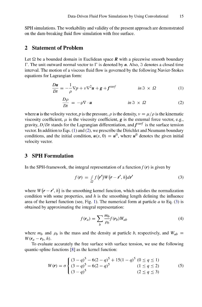
Let be a bounded domain in Euclidean space R with a piecewise smooth boundary
. The unit outward normal vector to is denoted by n. Also, denotes a closed time
interval. The motion of a viscous fluid flow is governed by the following Navier-Stokes
equations for Lagrangian form:
Du
Dt
= −
1
ρ
∇p + ν∇
2 u + g + f
surf
in × Ω
(1)
Dρ
Dt
= −ρ∇ · u
in × Ω
(2)
where u is the velocity vector, p is the pressure, ρ is the density, ν = μ/ρ is the kinematic
viscosity coefficient, μ is the viscosity coefficient, g is the external force vector, e.g.,
gravity, D/Dt stands for the Lagrangian differentiation, and f
surf is the surface tension
vector. In addition to Eqs. (1) and (2), we prescribe the Dirichlet and Neumann boundary
conditions, and the initial condition, u(x, 0) = u 0 , where u 0 denotes the given initial
velocity vector.
3 SPH Formulation
In the SPH-framework, the integral representation of a function f (r) is given by
f (r) = ∫
Ω
f
r
W
r − r
, h
d r
(3)
where W
r − r , h
is the smoothing kernel function, which satisfies the normalization
condition with some properties, and h is the smoothing length defining the influence
area of the kernel function (see, Fig. 1). The numerical form at particle a to Eq. (3) is
obtained by approximating the integral representation:
f (r a ) =
b
m b
ρ b
f (r b )W ab
(4)
where m b and ρ b is the mass and the density at particle b, respectively, and W ab =
W (r a − r b , h).
To evaluate accurately the free surface with surface tension, we use the following
quantic-spline functions [8] as the kernel function:
W (r) = σ
⎧
⎨
⎩
(3 − q)
5
− 6(2 − q)
5
+ 15(1 − q)
5
(0 ≤ q ≤ 1)
(3 − q)
5
− 6(2 − q)
5
(1 ≤ q ≤ 2)
(3 − q)
5
(2 ≤ q ≤ 3)
(5)
15
SPH simulations. The workability and validity of the present approach are demonstrated
on the dam-breaking fluid flow simulation with free surface.
2 Statement of Problem
Let be a bounded domain in Euclidean space R with a piecewise smooth boundary
. The unit outward normal vector to is denoted by n. Also, denotes a closed time
interval. The motion of a viscous fluid flow is governed by the following Navier-Stokes
equations for Lagrangian form:
Du
Dt
= −
1
ρ
∇p + ν∇
2 u + g + f
surf
in × Ω
(1)
Dρ
Dt
= −ρ∇ · u
in × Ω
(2)
where u is the velocity vector, p is the pressure, ρ is the density, ν = μ/ρ is the kinematic
viscosity coefficient, μ is the viscosity coefficient, g is the external force vector, e.g.,
gravity, D/Dt stands for the Lagrangian differentiation, and f
surf is the surface tension
vector. In addition to Eqs. (1) and (2), we prescribe the Dirichlet and Neumann boundary
conditions, and the initial condition, u(x, 0) = u 0 , where u 0 denotes the given initial
velocity vector.
3 SPH Formulation
In the SPH-framework, the integral representation of a function f (r) is given by
f (r) = ∫
Ω
f
r
W
r − r
, h
d r
(3)
where W
r − r , h
is the smoothing kernel function, which satisfies the normalization
condition with some properties, and h is the smoothing length defining the influence
area of the kernel function (see, Fig. 1). The numerical form at particle a to Eq. (3) is
obtained by approximating the integral representation:
f (r a ) =
b
m b
ρ b
f (r b )W ab
(4)
where m b and ρ b is the mass and the density at particle b, respectively, and W ab =
W (r a − r b , h).
To evaluate accurately the free surface with surface tension, we use the following
quantic-spline functions [8] as the kernel function:
W (r) = σ
⎧
⎨
⎩
(3 − q)
5
− 6(2 − q)
5
+ 15(1 − q)
5
(0 ≤ q ≤ 1)
(3 − q)
5
− 6(2 − q)
5
(1 ≤ q ≤ 2)
(3 − q)
5
(2 ≤ q ≤ 3)
(5)