

A New Locking-Free Thick/Thin Shell Element
105
u
P t
¯
α
P
1 , ¯
α
P
2 , α
P
3
≈ λ
b N
t
¯
α
P
1 , ¯
α
P
2 , α
P
3
a
b
;
(30)
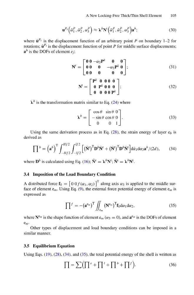
where ¯
u P r is the displacement function of an arbitrary point P on boundary 1–2 for
rotations; ¯
u P t is the displacement function of point P for middle surface displacements;
a b is the DOFs of element e j ;
N
r
=
⎡
⎣
0 0 −α 3 P k
0 0
0 0 0 −α 3 P k 0
0 0 0
0 0
⎤
⎦ ;
(31)
N
t
=
⎡
⎣
P k 0 0 0 0
0 P k 0 0 0
0 0 0 0 P k
⎤
⎦ ;
(32)
λ
b is the transformation matrix similar to Eq. (24) where
λ
b
=
⎡
⎣
cos θ sin θ 0
− sin θ cos θ 0
0
0 1
⎤
⎦ .
(33)
Using the same derivation process as in Eq. (28), the strain energy of layer e b is
derived as
b
=
a
b
T
H / 2
−H / 2
l / 2
−l / 2
¯
N
r
T D
b ¯
N
r
+
¯
N
t
T D
b ¯
N
t
d ¯
α 1 dα 3 a
b
/(2d ),
(34)
where D b is calculated using Eq. (16); ¯
N r = λ
b N r ; ¯
N t = λ
b N t .
3.4 Imposition of the Load Boundary Condition
A distributed force f 0 =
0 0 f (α 1 , α 2 )
T along axis α 3 is applied to the middle surface of element e m . Using Eq. (9), the external force potential energy of element e m is
expressed as
f
= −
a
e m
T
¨
e m
N
e m
T f 0 dα 1 dα 2 ,
(35)
where N e m is the shape function of element e m (α 3 = 0), and a e m is the DOFs of element
e m .
Other types of displacement and load boundary conditions can be imposed in a
similar manner.
3.5 Equilibrium Equation
Using Eqs. (19), (28), (34), and (35), the total potential energy of the shell is written as
=
e
+
l
+
b
+
f
.
(36)
105
u
P t
¯
α
P
1 , ¯
α
P
2 , α
P
3
≈ λ
b N
t
¯
α
P
1 , ¯
α
P
2 , α
P
3
a
b
;
(30)
where ¯
u P r is the displacement function of an arbitrary point P on boundary 1–2 for
rotations; ¯
u P t is the displacement function of point P for middle surface displacements;
a b is the DOFs of element e j ;
N
r
=
⎡
⎣
0 0 −α 3 P k
0 0
0 0 0 −α 3 P k 0
0 0 0
0 0
⎤
⎦ ;
(31)
N
t
=
⎡
⎣
P k 0 0 0 0
0 P k 0 0 0
0 0 0 0 P k
⎤
⎦ ;
(32)
λ
b is the transformation matrix similar to Eq. (24) where
λ
b
=
⎡
⎣
cos θ sin θ 0
− sin θ cos θ 0
0
0 1
⎤
⎦ .
(33)
Using the same derivation process as in Eq. (28), the strain energy of layer e b is
derived as
b
=
a
b
T
H / 2
−H / 2
l / 2
−l / 2
¯
N
r
T D
b ¯
N
r
+
¯
N
t
T D
b ¯
N
t
d ¯
α 1 dα 3 a
b
/(2d ),
(34)
where D b is calculated using Eq. (16); ¯
N r = λ
b N r ; ¯
N t = λ
b N t .
3.4 Imposition of the Load Boundary Condition
A distributed force f 0 =
0 0 f (α 1 , α 2 )
T along axis α 3 is applied to the middle surface of element e m . Using Eq. (9), the external force potential energy of element e m is
expressed as
f
= −
a
e m
T
¨
e m
N
e m
T f 0 dα 1 dα 2 ,
(35)
where N e m is the shape function of element e m (α 3 = 0), and a e m is the DOFs of element
e m .
Other types of displacement and load boundary conditions can be imposed in a
similar manner.
3.5 Equilibrium Equation
Using Eqs. (19), (28), (34), and (35), the total potential energy of the shell is written as
=
e
+
l
+
b
+
f
.
(36)