

A New Locking-Free Thick/Thin Shell Element
103
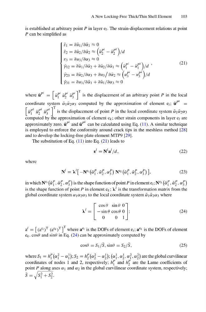
is established at arbitrary point P in layer e l . The strain-displacement relations at point
P can be simplified as
⎧
⎪ ⎪ ⎪ ⎪ ⎪ ⎪ ⎪ ⎪ ⎪ ⎨
⎪ ⎪ ⎪ ⎪ ⎪ ⎪ ⎪ ⎪ ⎪ ⎩
¯
ε 1 = ∂ ¯
u 1 /∂ ¯
α 1 ≈ 0
¯
ε 2 = ∂ ¯
u 2 /∂ ¯
α 2 ≈
¯
u P i
2 − ¯
u P k
2
/d
ε 3 = ∂u 3 /∂α 3 ≈ 0
¯
γ 12 = ∂ ¯
u 1 /∂ ¯
α 2 + ∂ ¯
u 2 /∂ ¯
α 1 ≈
¯
u P i
1 − ¯
u P k
1
/d
¯
γ 23 = ∂ ¯
u 2 /∂α 3 + ∂u 3
∂ ¯
α 2 ≈
u P i
3 − u P k
3
/d
¯
γ 31 = ∂u 3 /∂ ¯
α 1 + ∂ ¯
u 1 /∂α 3 ≈ 0
,
(21)
where ¯
u P i =
¯
u P i
1 ¯
u P i
2 ¯
u P i
3
T
is the displacement of an arbitrary point P in the local
coordinate system ¯
α 1 ¯
α 2 α 3 computed by the approximation of element e i ; ¯
u P k =
¯
u P k
1 ¯
u P k
2 ¯
u P k
3
T
is the displacement of point P in the local coordinate system ¯
α 1 ¯
α 2 α 3
computed by the approximation of element e k ; other strain components in layer e l are
approximately zero. ¯
u P i and ¯
u P k can be calculated using Eq. (11). A similar technique
is employed to enforce the conformity around crack tips in the meshless method [28]
and to develop the locking-free plate element MTP9 [29].
The substitution of Eq. (11) into Eq. (21) leads to
ε
l
= N
l a
l
/d ,
(22)
where
N
l
= λ
l
−N e i
¯
α P
1 , ¯
α P
2 , α P
3
N e k
¯
α P
1 , ¯
α P
2 , α P
3
,
(23)
in which N e i
¯
α P
1 , ¯
α P
2 , α P
3
is the shape function of point P in element e i ; N e k
¯
α P
1 , ¯
α P
2 , α P
3
is the shape function of point P in element e k ; λ
l is the transformation matrix from the
global coordinate system α 1 α 2 α 3 to the local coordinate system ¯
α 1 ¯
α 2 α 3 where
λ
l
=
⎡
⎣
cos θ sin θ 0
− sin θ cos θ 0
0
0 1
⎤
⎦ ;
(24)
a l =
(a e i )
T
(a e k )
T
T where a e i is the DOFs of element e i ; a e k is the DOFs of element
e k . cosθ and sinθ in Eq. (24) can be approximately computed by
cosθ = S 1 / ¯
S, sinθ = S 2 / ¯
S,
(25)
where S 1 = h P
1
α 2
1 − α 1
1
; S 2 = h P
2
α 2
2 − α 1
2
;
α 1
1 , α 1
2 , α 2
1 , α 2
2
are the global curvilinear
coordinates of nodes 1 and 2, respectively; h P
1 and h P
2 are the Lame coefficients of
point P along axes α 1 and α 2 in the global curvilinear coordinate system, respectively;
¯
S =
S 2
1 + S 2
2 .
103
is established at arbitrary point P in layer e l . The strain-displacement relations at point
P can be simplified as
⎧
⎪ ⎪ ⎪ ⎪ ⎪ ⎪ ⎪ ⎪ ⎪ ⎨
⎪ ⎪ ⎪ ⎪ ⎪ ⎪ ⎪ ⎪ ⎪ ⎩
¯
ε 1 = ∂ ¯
u 1 /∂ ¯
α 1 ≈ 0
¯
ε 2 = ∂ ¯
u 2 /∂ ¯
α 2 ≈
¯
u P i
2 − ¯
u P k
2
/d
ε 3 = ∂u 3 /∂α 3 ≈ 0
¯
γ 12 = ∂ ¯
u 1 /∂ ¯
α 2 + ∂ ¯
u 2 /∂ ¯
α 1 ≈
¯
u P i
1 − ¯
u P k
1
/d
¯
γ 23 = ∂ ¯
u 2 /∂α 3 + ∂u 3
∂ ¯
α 2 ≈
u P i
3 − u P k
3
/d
¯
γ 31 = ∂u 3 /∂ ¯
α 1 + ∂ ¯
u 1 /∂α 3 ≈ 0
,
(21)
where ¯
u P i =
¯
u P i
1 ¯
u P i
2 ¯
u P i
3
T
is the displacement of an arbitrary point P in the local
coordinate system ¯
α 1 ¯
α 2 α 3 computed by the approximation of element e i ; ¯
u P k =
¯
u P k
1 ¯
u P k
2 ¯
u P k
3
T
is the displacement of point P in the local coordinate system ¯
α 1 ¯
α 2 α 3
computed by the approximation of element e k ; other strain components in layer e l are
approximately zero. ¯
u P i and ¯
u P k can be calculated using Eq. (11). A similar technique
is employed to enforce the conformity around crack tips in the meshless method [28]
and to develop the locking-free plate element MTP9 [29].
The substitution of Eq. (11) into Eq. (21) leads to
ε
l
= N
l a
l
/d ,
(22)
where
N
l
= λ
l
−N e i
¯
α P
1 , ¯
α P
2 , α P
3
N e k
¯
α P
1 , ¯
α P
2 , α P
3
,
(23)
in which N e i
¯
α P
1 , ¯
α P
2 , α P
3
is the shape function of point P in element e i ; N e k
¯
α P
1 , ¯
α P
2 , α P
3
is the shape function of point P in element e k ; λ
l is the transformation matrix from the
global coordinate system α 1 α 2 α 3 to the local coordinate system ¯
α 1 ¯
α 2 α 3 where
λ
l
=
⎡
⎣
cos θ sin θ 0
− sin θ cos θ 0
0
0 1
⎤
⎦ ;
(24)
a l =
(a e i )
T
(a e k )
T
T where a e i is the DOFs of element e i ; a e k is the DOFs of element
e k . cosθ and sinθ in Eq. (24) can be approximately computed by
cosθ = S 1 / ¯
S, sinθ = S 2 / ¯
S,
(25)
where S 1 = h P
1
α 2
1 − α 1
1
; S 2 = h P
2
α 2
2 − α 1
2
;
α 1
1 , α 1
2 , α 2
1 , α 2
2
are the global curvilinear
coordinates of nodes 1 and 2, respectively; h P
1 and h P
2 are the Lame coefficients of
point P along axes α 1 and α 2 in the global curvilinear coordinate system, respectively;
¯
S =
S 2
1 + S 2
2 .