

506
R. Ahrens et al.
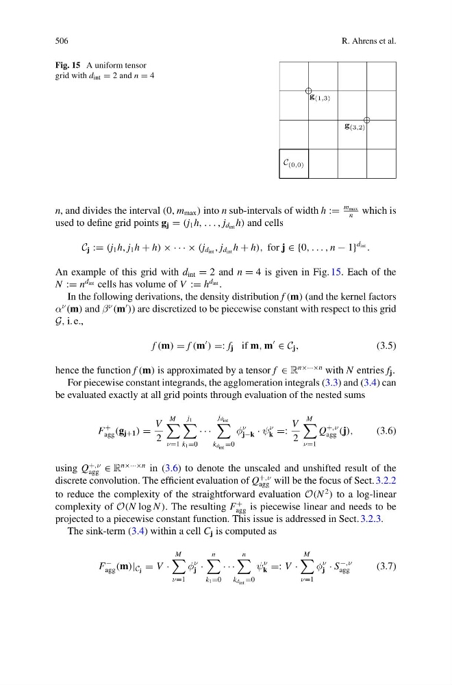
Fig. 15 A uniform tensor
grid with d int = 2 and n = 4
C (0,0)
g (1,3)
g (3,2)
n, and divides the interval (0, m max ) into n sub-intervals of width h :=
m max
n
which is
used to define grid points g j = (j 1 h, . . . , j d int h) and cells
C j := (j 1 h, j 1 h + h) × · · · × (j d int , j d int h + h), for j ∈ {0, . . . , n − 1}
d int .
An example of this grid with d int = 2 and n = 4 is given in Fig. 15. Each of the
N := n
d int cells has volume of V := h
d int .
In the following derivations, the density distribution f (m) (and the kernel factors
α
ν
(m) and β
ν
(m
)) are discretized to be piecewise constant with respect to this grid
G, i. e.,
f (m) = f (m
) =: f j if m, m
∈ C j ,
(3.5)
hence the function f (m) is approximated by a tensor f ∈ R
n×···×n with N entries f j .
For piecewise constant integrands, the agglomeration integrals (3.3) and (3.4) can
be evaluated exactly at all grid points through evaluation of the nested sums
F
+
agg (g j+1 ) =
V
2
M
ν=1
j 1
k 1 =0
· · ·
j d int
k d int =0
φ
ν
j−k · ψ
ν
k =:
V
2
M
ν=1
Q
+,ν
agg (j),
(3.6)
using Q
+,ν
agg ∈ R
n×···×n in (3.6) to denote the unscaled and unshifted result of the
discrete convolution. The efficient evaluation of Q
+,ν
agg will be the focus of Sect. 3.2.2
to reduce the complexity of the straightforward evaluation O(N
2
) to a log-linear
complexity of O(N log N ). The resulting F
+
agg is piecewise linear and needs to be
projected to a piecewise constant function. This issue is addressed in Sect. 3.2.3.
The sink-term (3.4) within a cell C j is computed as
F
−
agg (m)| C j = V ·
M
ν=1
φ
ν
j ·
n
k 1 =0
· · ·
n
k d int =0
ψ
ν
k =: V ·
M
ν=1
φ
ν
j · S
−,ν
agg
(3.7)
R. Ahrens et al.
Fig. 15 A uniform tensor
grid with d int = 2 and n = 4
C (0,0)
g (1,3)
g (3,2)
n, and divides the interval (0, m max ) into n sub-intervals of width h :=
m max
n
which is
used to define grid points g j = (j 1 h, . . . , j d int h) and cells
C j := (j 1 h, j 1 h + h) × · · · × (j d int , j d int h + h), for j ∈ {0, . . . , n − 1}
d int .
An example of this grid with d int = 2 and n = 4 is given in Fig. 15. Each of the
N := n
d int cells has volume of V := h
d int .
In the following derivations, the density distribution f (m) (and the kernel factors
α
ν
(m) and β
ν
(m
)) are discretized to be piecewise constant with respect to this grid
G, i. e.,
f (m) = f (m
) =: f j if m, m
∈ C j ,
(3.5)
hence the function f (m) is approximated by a tensor f ∈ R
n×···×n with N entries f j .
For piecewise constant integrands, the agglomeration integrals (3.3) and (3.4) can
be evaluated exactly at all grid points through evaluation of the nested sums
F
+
agg (g j+1 ) =
V
2
M
ν=1
j 1
k 1 =0
· · ·
j d int
k d int =0
φ
ν
j−k · ψ
ν
k =:
V
2
M
ν=1
Q
+,ν
agg (j),
(3.6)
using Q
+,ν
agg ∈ R
n×···×n in (3.6) to denote the unscaled and unshifted result of the
discrete convolution. The efficient evaluation of Q
+,ν
agg will be the focus of Sect. 3.2.2
to reduce the complexity of the straightforward evaluation O(N
2
) to a log-linear
complexity of O(N log N ). The resulting F
+
agg is piecewise linear and needs to be
projected to a piecewise constant function. This issue is addressed in Sect. 3.2.3.
The sink-term (3.4) within a cell C j is computed as
F
−
agg (m)| C j = V ·
M
ν=1
φ
ν
j ·
n
k 1 =0
· · ·
n
k d int =0
ψ
ν
k =: V ·
M
ν=1
φ
ν
j · S
−,ν
agg
(3.7)