

15.8 Random Response of SDF Systems
545
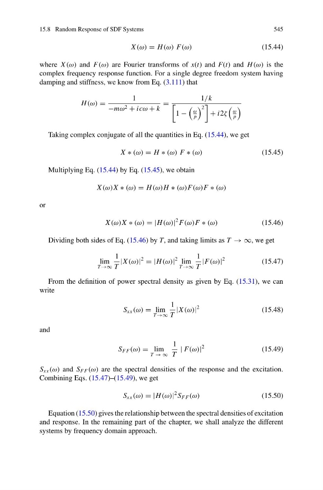
X (ω) = H (ω) F(ω)
(15.44)
where X (ω) and F(ω) are Fourier transforms of x(t) and F(t) and H (ω) is the
complex frequency response function. For a single degree freedom system having
damping and stiffness, we know from Eq. (3.111) that
H (ω) =
1
−mω 2 + icω + k
=
1/k
1 −
ω
p
2
+ i2ζ
ω
p
Taking complex conjugate of all the quantities in Eq. (15.44), we get
X ∗ (ω) = H ∗ (ω) F ∗ (ω)
(15.45)
Multiplying Eq. (15.44) by Eq. (15.45), we obtain
X (ω)X ∗ (ω) = H (ω)H ∗ (ω)F(ω)F ∗ (ω)
or
X (ω)X ∗ (ω) = |H (ω)|
2 F(ω)F ∗ (ω)
(15.46)
Dividing both sides of Eq. (15.46) by T, and taking limits as T → ∞, we get
lim
T →∞
1
T
|X (ω)|
2
= |H (ω)|
2 lim
T →∞
1
T
|F(ω)|
2
(15.47)
From the definition of power spectral density as given by Eq. (15.31), we can
write
S xx (ω) = lim
T →∞
1
T
|X (ω)|
2
(15.48)
and
S F F (ω) = lim
T → ∞
1
T
| F(ω)|
2
(15.49)
S xx (ω) and S F F (ω) are the spectral densities of the response and the excitation.
Combining Eqs. (15.47)–(15.49), we get
S xx (ω) = |H (ω)|
2 S F F (ω)
(15.50)
Equation (15.50) gives the relationship between the spectral densities of excitation
and response. In the remaining part of the chapter, we shall analyze the different
systems by frequency domain approach.
545
X (ω) = H (ω) F(ω)
(15.44)
where X (ω) and F(ω) are Fourier transforms of x(t) and F(t) and H (ω) is the
complex frequency response function. For a single degree freedom system having
damping and stiffness, we know from Eq. (3.111) that
H (ω) =
1
−mω 2 + icω + k
=
1/k
1 −
ω
p
2
+ i2ζ
ω
p
Taking complex conjugate of all the quantities in Eq. (15.44), we get
X ∗ (ω) = H ∗ (ω) F ∗ (ω)
(15.45)
Multiplying Eq. (15.44) by Eq. (15.45), we obtain
X (ω)X ∗ (ω) = H (ω)H ∗ (ω)F(ω)F ∗ (ω)
or
X (ω)X ∗ (ω) = |H (ω)|
2 F(ω)F ∗ (ω)
(15.46)
Dividing both sides of Eq. (15.46) by T, and taking limits as T → ∞, we get
lim
T →∞
1
T
|X (ω)|
2
= |H (ω)|
2 lim
T →∞
1
T
|F(ω)|
2
(15.47)
From the definition of power spectral density as given by Eq. (15.31), we can
write
S xx (ω) = lim
T →∞
1
T
|X (ω)|
2
(15.48)
and
S F F (ω) = lim
T → ∞
1
T
| F(ω)|
2
(15.49)
S xx (ω) and S F F (ω) are the spectral densities of the response and the excitation.
Combining Eqs. (15.47)–(15.49), we get
S xx (ω) = |H (ω)|
2 S F F (ω)
(15.50)
Equation (15.50) gives the relationship between the spectral densities of excitation
and response. In the remaining part of the chapter, we shall analyze the different
systems by frequency domain approach.