

420
10 Dynamic Direct Stiffness Method
{δ} e =
⎧
⎪ ⎪ ⎨
⎪ ⎪ ⎩
ψ i
ψ j
Y i
Y j
⎫
⎪ ⎪ ⎬
⎪ ⎪ ⎭
(10.100)
and
{P} e =
⎧
⎪ ⎪ ⎨
⎪ ⎪ ⎩
M i
M j
V i
V j
⎫
⎪ ⎪ ⎬
⎪ ⎪ ⎭
(10.101)
With the help of Eq. (10.92), the nodal displacements can be related to the
constants. They are expressed in matrix form as
{δ} e = [G]{C}
(10.102)
Similarly, with the help of Eq. (10.95), nodal forces can be expressed in terms of
constants as
{P} e = [H ]{C}
(10.103)
Eliminating {C} between Eqs. (10.102) and (10.103), we get
{P} e = [H ][G]
−1
{δ} e
or
{P} e = [K ]{δ} e
(10.104)
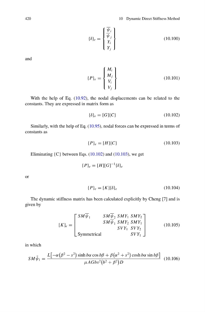
The dynamic stiffness matrix has been calculated explicitly by Cheng [7] and is
given by
[K ] e =
⎡
⎢
⎢
⎣
SMψ 1
SMψ 2 SMY 1 SMY 2
SMψ 1 SMY 2 SMY 1
SV Y 1 SV Y 2
Symmetrical
SV Y 1
⎤
⎥
⎥
⎦
(10.105)
in which
SM ¯
ψ 1 =
L
−α
β
2
− s
2
sinh bα cos bβ + β
α
2
+ s
2
cosh bα sin bβ
μAGbs 2
b 2 + β 2
D
(10.106)
10 Dynamic Direct Stiffness Method
{δ} e =
⎧
⎪ ⎪ ⎨
⎪ ⎪ ⎩
ψ i
ψ j
Y i
Y j
⎫
⎪ ⎪ ⎬
⎪ ⎪ ⎭
(10.100)
and
{P} e =
⎧
⎪ ⎪ ⎨
⎪ ⎪ ⎩
M i
M j
V i
V j
⎫
⎪ ⎪ ⎬
⎪ ⎪ ⎭
(10.101)
With the help of Eq. (10.92), the nodal displacements can be related to the
constants. They are expressed in matrix form as
{δ} e = [G]{C}
(10.102)
Similarly, with the help of Eq. (10.95), nodal forces can be expressed in terms of
constants as
{P} e = [H ]{C}
(10.103)
Eliminating {C} between Eqs. (10.102) and (10.103), we get
{P} e = [H ][G]
−1
{δ} e
or
{P} e = [K ]{δ} e
(10.104)
The dynamic stiffness matrix has been calculated explicitly by Cheng [7] and is
given by
[K ] e =
⎡
⎢
⎢
⎣
SMψ 1
SMψ 2 SMY 1 SMY 2
SMψ 1 SMY 2 SMY 1
SV Y 1 SV Y 2
Symmetrical
SV Y 1
⎤
⎥
⎥
⎦
(10.105)
in which
SM ¯
ψ 1 =
L
−α
β
2
− s
2
sinh bα cos bβ + β
α
2
+ s
2
cosh bα sin bβ
μAGbs 2
b 2 + β 2
D
(10.106)