

6.21 Component Mode Synthesis Method
249
[K ]
S
= [φ ]
T
N [K ]
S
[φ ] N
(6.189)
Both [M]
S and [K ]
S are diagonal matrices.
Putting
[M] S = [I ]
(6.190)
and
[K ] S =
1/ p
2
r
S
(6.191)
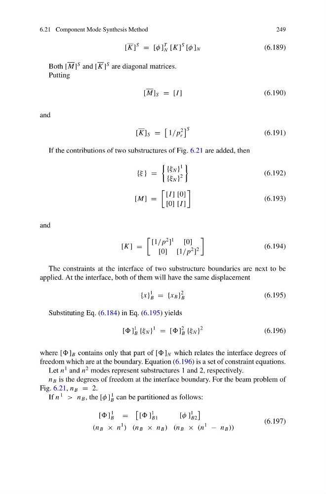
If the contributions of two substructures of Fig. 6.21 are added, then
{ξ } =
{ξ N }
1
{ξ N }
2
(6.192)
[M] =
[I ] [0]
[0] [I ]
(6.193)
and
[K ] =
[1/ p
2
]
1
[0]
[0] [1/ p
2
]
2
(6.194)
The constraints at the interface of two substructure boundaries are next to be
applied. At the interface, both of them will have the same displacement
{x}
1
B = {x B }
2
B
(6.195)
Substituting Eq. (6.184) in Eq. (6.195) yields
[ ]
1
B {ξ N }
1
= [ ]
2
B {ξ N }
2
(6.196)
where [ ] B contains only that part of [ ] N which relates the interface degrees of
freedom which are at the boundary. Equation (6.196) is a set of constraint equations.
Let n
1 and n
2 modes represent substructures 1 and 2, respectively.
n B is the degrees of freedom at the interface boundary. For the beam problem of
Fig. 6.21, n B = 2.
If n
1
> n B , the [φ ]
1
B can be partitioned as follows:
[ ]
1
B
=
[ ]
1
B1
[φ ]
1
B2
(n B × n
1
) (n B × n B ) (n B × (n
1
− n B ))
(6.197)
249
[K ]
S
= [φ ]
T
N [K ]
S
[φ ] N
(6.189)
Both [M]
S and [K ]
S are diagonal matrices.
Putting
[M] S = [I ]
(6.190)
and
[K ] S =
1/ p
2
r
S
(6.191)
If the contributions of two substructures of Fig. 6.21 are added, then
{ξ } =
{ξ N }
1
{ξ N }
2
(6.192)
[M] =
[I ] [0]
[0] [I ]
(6.193)
and
[K ] =
[1/ p
2
]
1
[0]
[0] [1/ p
2
]
2
(6.194)
The constraints at the interface of two substructure boundaries are next to be
applied. At the interface, both of them will have the same displacement
{x}
1
B = {x B }
2
B
(6.195)
Substituting Eq. (6.184) in Eq. (6.195) yields
[ ]
1
B {ξ N }
1
= [ ]
2
B {ξ N }
2
(6.196)
where [ ] B contains only that part of [ ] N which relates the interface degrees of
freedom which are at the boundary. Equation (6.196) is a set of constraint equations.
Let n
1 and n
2 modes represent substructures 1 and 2, respectively.
n B is the degrees of freedom at the interface boundary. For the beam problem of
Fig. 6.21, n B = 2.
If n
1
> n B , the [φ ]
1
B can be partitioned as follows:
[ ]
1
B
=
[ ]
1
B1
[φ ]
1
B2
(n B × n
1
) (n B × n B ) (n B × (n
1
− n B ))
(6.197)