

6.12 Stodola’s Method
221
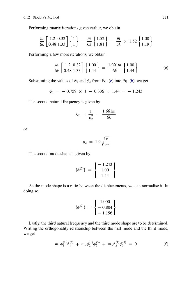
Performing matrix iterations given earlier, we obtain
m
6k
1.2 0.32
0.48 1.33
1
1
=
m
6k
1.52
1.81
=
m
6k
× 1.52
1.00
1.19
Performing a few more iterations, we obtain
m
6k
1.2 0.32
0.48 1.33
1.00
1.44
=
1.661m
6k
1.00
1.44
(e)
Substituting the values of φ 2 and φ 3 from Eq. (e) into Eq. (b), we get
φ 1 = − 0.759 × 1 − 0.336 × 1.44 = − 1.243
The second natural frequency is given by
λ 2 =
1
p
2
2
=
1.661m
6k
or
p 2 = 1.9
k
m
The second mode shape is given by
{φ
(2)
} =
⎧
⎨
⎩
− 1.243
1.00
1.44
⎫
⎬
⎭
As the mode shape is a ratio between the displacements, we can normalise it. In
doing so
{φ
(2)
} =
⎧
⎨
⎩
1.000
− 0.804
− 1.156
⎫
⎬
⎭
Lastly, the third natural frequency and the third mode shape are to be determined.
Writing the orthogonality relationship between the first mode and the third mode,
we get
m 1 φ
(1)
1 φ
(3)
1
+ m 2 φ
(1)
2 φ
(3)
2
+ m 3 φ
(1)
3 φ
(3)
3
= 0
( f )
221
Performing matrix iterations given earlier, we obtain
m
6k
1.2 0.32
0.48 1.33
1
1
=
m
6k
1.52
1.81
=
m
6k
× 1.52
1.00
1.19
Performing a few more iterations, we obtain
m
6k
1.2 0.32
0.48 1.33
1.00
1.44
=
1.661m
6k
1.00
1.44
(e)
Substituting the values of φ 2 and φ 3 from Eq. (e) into Eq. (b), we get
φ 1 = − 0.759 × 1 − 0.336 × 1.44 = − 1.243
The second natural frequency is given by
λ 2 =
1
p
2
2
=
1.661m
6k
or
p 2 = 1.9
k
m
The second mode shape is given by
{φ
(2)
} =
⎧
⎨
⎩
− 1.243
1.00
1.44
⎫
⎬
⎭
As the mode shape is a ratio between the displacements, we can normalise it. In
doing so
{φ
(2)
} =
⎧
⎨
⎩
1.000
− 0.804
− 1.156
⎫
⎬
⎭
Lastly, the third natural frequency and the third mode shape are to be determined.
Writing the orthogonality relationship between the first mode and the third mode,
we get
m 1 φ
(1)
1 φ
(3)
1
+ m 2 φ
(1)
2 φ
(3)
2
+ m 3 φ
(1)
3 φ
(3)
3
= 0
( f )