

6.12 Stodola’s Method
219
[D] = [K ]
− 1
[M] =
1
6k
⎡
⎣
8 5 2
5 5 2
2 2 2
⎤
⎦ m
⎡
⎣
1 0 0
0 1 0
0 0 1
⎤
⎦ =
m
6k
⎡
⎣
8 5 2
5 5 2
2 2 2
⎤
⎦
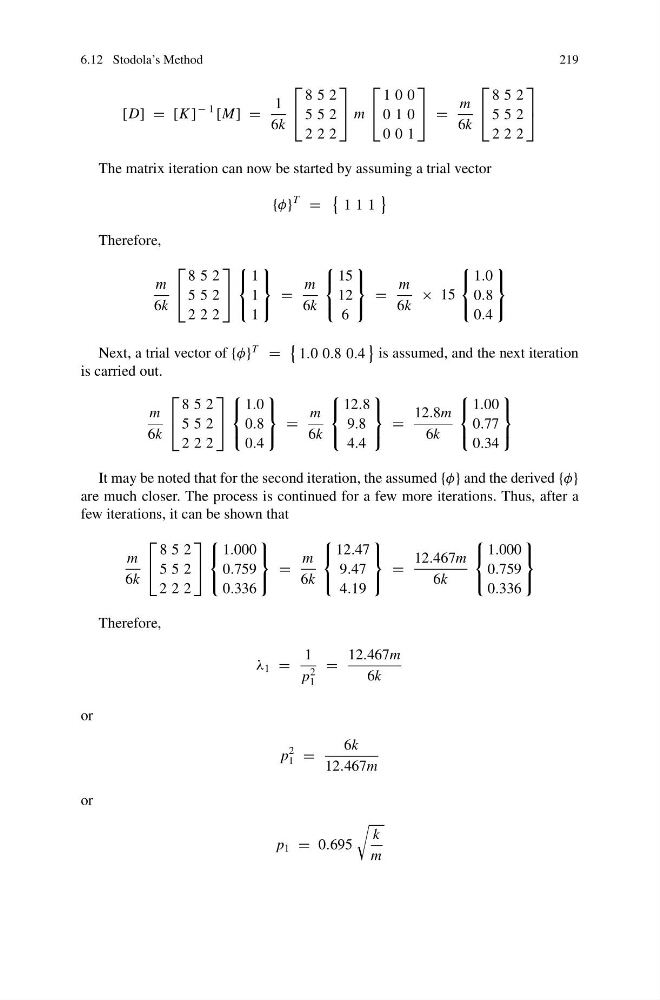
The matrix iteration can now be started by assuming a trial vector
{φ}
T
=
1 1 1
Therefore,
m
6k
⎡
⎣
8 5 2
5 5 2
2 2 2
⎤
⎦
⎧
⎨
⎩
1
1
1
⎫
⎬
⎭
=
m
6k
⎧
⎨
⎩
15
12
6
⎫
⎬
⎭
=
m
6k
× 15
⎧
⎨
⎩
1.0
0.8
0.4
⎫
⎬
⎭
Next, a trial vector of {φ}
T
=
1.0 0.8 0.4
is assumed, and the next iteration
is carried out.
m
6k
⎡
⎣
8 5 2
5 5 2
2 2 2
⎤
⎦
⎧
⎨
⎩
1.0
0.8
0.4
⎫
⎬
⎭
=
m
6k
⎧
⎨
⎩
12.8
9.8
4.4
⎫
⎬
⎭
=
12.8m
6k
⎧
⎨
⎩
1.00
0.77
0.34
⎫
⎬
⎭
It may be noted that for the second iteration, the assumed {φ} and the derived {φ}
are much closer. The process is continued for a few more iterations. Thus, after a
few iterations, it can be shown that
m
6k
⎡
⎣
8 5 2
5 5 2
2 2 2
⎤
⎦
⎧
⎨
⎩
1.000
0.759
0.336
⎫
⎬
⎭
=
m
6k
⎧
⎨
⎩
12.47
9.47
4.19
⎫
⎬
⎭
=
12.467m
6k
⎧
⎨
⎩
1.000
0.759
0.336
⎫
⎬
⎭
Therefore,
λ 1 =
1
p
2
1
=
12.467m
6k
or
p
2
1 =
6k
12.467m
or
p 1 = 0.695
k
m
219
[D] = [K ]
− 1
[M] =
1
6k
⎡
⎣
8 5 2
5 5 2
2 2 2
⎤
⎦ m
⎡
⎣
1 0 0
0 1 0
0 0 1
⎤
⎦ =
m
6k
⎡
⎣
8 5 2
5 5 2
2 2 2
⎤
⎦
The matrix iteration can now be started by assuming a trial vector
{φ}
T
=
1 1 1
Therefore,
m
6k
⎡
⎣
8 5 2
5 5 2
2 2 2
⎤
⎦
⎧
⎨
⎩
1
1
1
⎫
⎬
⎭
=
m
6k
⎧
⎨
⎩
15
12
6
⎫
⎬
⎭
=
m
6k
× 15
⎧
⎨
⎩
1.0
0.8
0.4
⎫
⎬
⎭
Next, a trial vector of {φ}
T
=
1.0 0.8 0.4
is assumed, and the next iteration
is carried out.
m
6k
⎡
⎣
8 5 2
5 5 2
2 2 2
⎤
⎦
⎧
⎨
⎩
1.0
0.8
0.4
⎫
⎬
⎭
=
m
6k
⎧
⎨
⎩
12.8
9.8
4.4
⎫
⎬
⎭
=
12.8m
6k
⎧
⎨
⎩
1.00
0.77
0.34
⎫
⎬
⎭
It may be noted that for the second iteration, the assumed {φ} and the derived {φ}
are much closer. The process is continued for a few more iterations. Thus, after a
few iterations, it can be shown that
m
6k
⎡
⎣
8 5 2
5 5 2
2 2 2
⎤
⎦
⎧
⎨
⎩
1.000
0.759
0.336
⎫
⎬
⎭
=
m
6k
⎧
⎨
⎩
12.47
9.47
4.19
⎫
⎬
⎭
=
12.467m
6k
⎧
⎨
⎩
1.000
0.759
0.336
⎫
⎬
⎭
Therefore,
λ 1 =
1
p
2
1
=
12.467m
6k
or
p
2
1 =
6k
12.467m
or
p 1 = 0.695
k
m