

6.10 Transfer Matrix Method
209
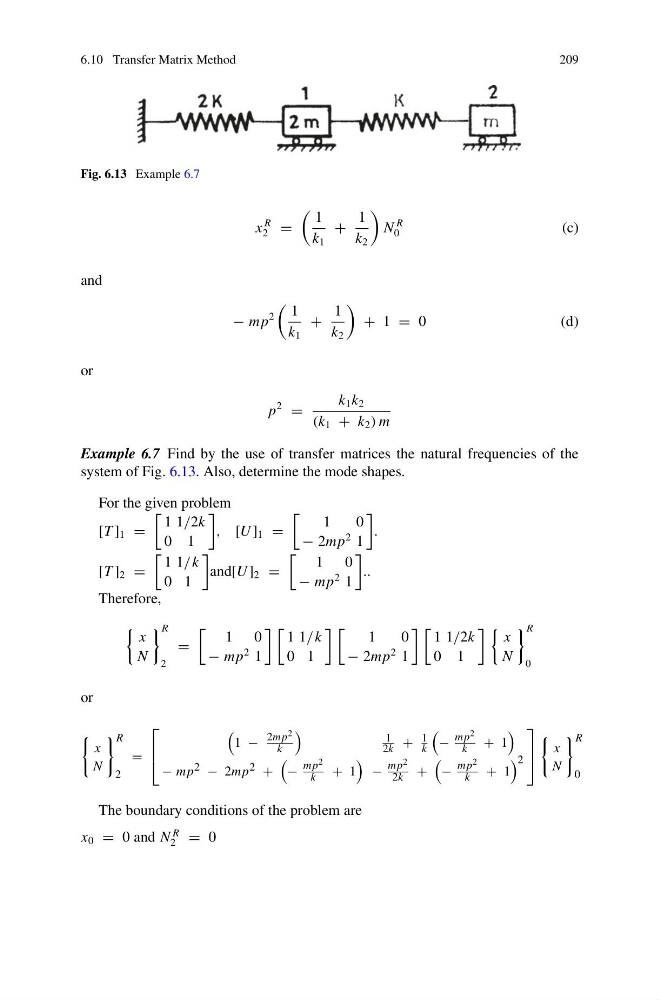
Fig. 6.13 Example 6.7
x
R
2 =
1
k 1
+
1
k 2
N
R
0
(c)
and
− mp
2
1
k 1
+
1
k 2
+ 1 = 0
( d )
or
p
2
=
k 1 k 2
(k 1 + k 2 ) m
Example 6.7 Find by the use of transfer matrices the natural frequencies of the
system of Fig. 6.13. Also, determine the mode shapes.
For the given problem
[T ] 1 =
1 1/2k
0 1
, [U ] 1 =
1
0
− 2mp
2 1
.
[T ] 2 =
1 1/k
0 1
and[U ] 2 =
1 0
− mp
2 1
..
Therefore,
x
N
R
2
=
1 0
− mp
2 1
1 1/k
0 1
1
0
− 2mp
2 1
1 1/2k
0 1
x
N
R
0
or
x
N
R
2
=
⎡
⎢
⎣
1 −
2mp 2
k
1
2k + 1
k
−
mp 2
k + 1
− mp 2 − 2mp 2 +
−
mp 2
k + 1
−
mp 2
2k +
−
mp 2
k + 1
2
⎤
⎥
⎦
x
N
R
0
The boundary conditions of the problem are
x 0 = 0 and N
R
2 = 0
209
Fig. 6.13 Example 6.7
x
R
2 =
1
k 1
+
1
k 2
N
R
0
(c)
and
− mp
2
1
k 1
+
1
k 2
+ 1 = 0
( d )
or
p
2
=
k 1 k 2
(k 1 + k 2 ) m
Example 6.7 Find by the use of transfer matrices the natural frequencies of the
system of Fig. 6.13. Also, determine the mode shapes.
For the given problem
[T ] 1 =
1 1/2k
0 1
, [U ] 1 =
1
0
− 2mp
2 1
.
[T ] 2 =
1 1/k
0 1
and[U ] 2 =
1 0
− mp
2 1
..
Therefore,
x
N
R
2
=
1 0
− mp
2 1
1 1/k
0 1
1
0
− 2mp
2 1
1 1/2k
0 1
x
N
R
0
or
x
N
R
2
=
⎡
⎢
⎣
1 −
2mp 2
k
1
2k + 1
k
−
mp 2
k + 1
− mp 2 − 2mp 2 +
−
mp 2
k + 1
−
mp 2
2k +
−
mp 2
k + 1
2
⎤
⎥
⎦
x
N
R
0
The boundary conditions of the problem are
x 0 = 0 and N
R
2 = 0